Splay trees
A balanced search tree is the foundation for many modern algorithms. On the pages of books on Computer Science, you will find descriptions of red-black, AVL-, B-, and many other balanced trees. But is the permanent balance the Holy Grail to be followed?
Imagine that we have already built a tree on keys and now we need to respond to requests whether the given key lies in the tree. It may well turn out that the user is mainly interested in one key, and he only requests the rest from time to time. If the key is far from the root, then
  requests can take away
  of time. Common sense suggests that the assessment can be optimized to
  by adding a cache over the tree. But this approach has some lack of flexibility and elegance.
Today I will talk about splay trees. These trees are not permanently balanced and even linear time can work on individual queries. However, after each request, they change their structure, which allows to process frequently repeated requests very effectively. Moreover, the depreciation cost of processing a single request from them , which makes splay-trees a good alternative for permanently balanced counterparts.
In the mid-eighties, Robert Taryan and Daniel Slaytor proposed some beautiful and effective data structures. All of them have a simple basic structure and one or two heuristics, which they constantly locally correct. A splay tree is one such structure.
')
A splay tree is a self-balancing binary search tree. The tree does not need to store any additional information, which makes it efficient in memory. After each conversion, even a search, the splay tree changes its structure.
Below I will describe the algorithm of how a tree works on a set of pairs of different keys, and then I will give its analysis.
To describe the structure of the tree, we need a simple class that describes a single vertex,
and two supporting procedures for working with parent signs.
The basic heuristic of a splay tree is move-to-root. After referring to any vertex, it rises to the root. The ascent is realized through the turns of the peaks. In one turn, you can swap the parent with the child, as shown in the figure below.

But simply turning the top until it becomes a root is not enough. The trick of a splay tree is that as the vertex moves up, the distance to the root is reduced not only for the lifted vertex, but also for all its descendants in the current subtrees. To do this, use the technique of zig-zig and zig-zag turns.
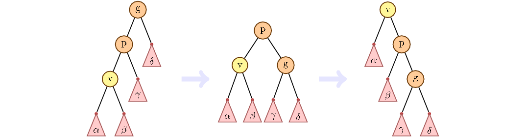
The main idea of zig-zig and zig-zag turns, to consider the path from grandfather to child. If the path goes only on the left children or only on the right, then this situation is called zig-zig. How to handle it is shown in the figure below. First turn the parent, then the child.
Otherwise, we first change the child with the current parent, then with the new one.

If the top of the grandfather is not, we make the usual turn:

The above procedure for raising vertices using zig-zig and zig-zag turns is key for a splay-tree.
Note In Russian, the term "splay" was translated as "expand." I think this is not a very good translation. You take the top and pull it up. At this time, all the other peaks go down, turning around it. Something similar happens when you twist the T-shirt. So the word "turn out" seems more appropriate here.
The search procedure in the splay-tree differs from the usual one only at the last stage: after the vertex is found, we pull it up and root it through the
To implement the insertion and deletion of the key, we need two procedures:
The
To insert the next key, it is enough to call
The
To remove a vertex, you need to lift it up, and then merge its left and right subtrees.
In order for a splay tree to support duplicate keys, you can proceed in two ways. It is necessary either to match each key with a list that stores the required add. information, or implement the find procedure so that it returns the first vertex in the LUR traversal order with the key greater or equal to the specified one.
Note that the procedures for deleting, inserting, merging and splitting trees work for + time of the
The
For the analysis we will use the method of the physicist, about which I told in the article about the depreciation analysis . Let be - subtree size
  with root at the top
  . Rank tops let's call the value
  . Our potential will be
  .
.
We assume that the actual time of the tops . Note that this is also equal to the number of elementary turns that will be performed during the procedure.
Approval The depreciation value of the in a tree  with root
  is up
is up  .
.
Proof .
If a - root, the statement is obvious. Otherwise, we divide the
After each stage the rank of the top will change. Let the rank initially be  , and then
  -th stage -
  . For each stage, except, perhaps, the last, we show that the amortization time for its execution can be limited from above by
  . For the last stage, the upper estimate will be
  . Summing the upper estimates and reducing the intermediate values of the ranks, we obtain the required

It only needs to be noted that , but
, but  .
.
Now we will analyze each type of rotation separately.
Zig. It can be performed only once, at the last stage. Actual time . Let's look at the picture and understand that only vertices change ranks. and .

So, the depreciation value will be . Ranks
  and
and  are shrinking. Based on the size of the respective subtrees, apply to the formula
  inequality:

So .
.
Zig-zig Actual time . Note that the ranks change only at the vertices.
  ,
,  and
and  .
.

Then the depreciation value . Ranks and can be cut. We get that
  . Based on the size of the subtrees applicable to the formula two inequalities:

and get that .
.
Our goal is to show that . To do this, it is enough to show that
  :
:

For convenience, we transfer the ranks to the left-hand side and prove . By definition rank
  . The last equality is divided by the sum
  . Let's look at the picture and understand that
  .
.
Fact for any positive
  such that
  .
.
So . Got the required.
Zig-zag.

Similar to the previous case, we write down the depreciation estimate: .
Ranks and are shrinking. To formula the following inequalities apply:

So . This inequality is proved in the same way as in the previous case.
Thus, we have analyzed all three cases and obtained the upper estimate for the amortized time through the ranks.
It remains to note that the rank of any vertex is limited by the logarithm of the size of the tree. Which implies the following theorem.
Theorem . The .
For dessert, I would like to refer to Wikipedia and present here some interesting facts about
Static optimality theorem . Let be - the number of times the item was requested
  . Then doing
  search queries on the
  .
.
In fact, this fact reports the following. Let us know in advance how many queries will be set for various elements. We build some specific binary tree to respond to these requests as quickly as possible. The statement says that, up to a constant
The current set theorem . Let be Is the number of requests that we have already made since the last request to the element
  ; if not already accessed, then just the number of requests from the beginning. Then the processing time requests will be
  .
.
This fact formalizes my reasoning about the cache at the beginning of the article. In fact, he says that, on average, the recently requested element does not float far from the root.
Scanning theorem Sequential access (LUR) to the elements of a .
.
This fact has a great practical implication. Together with the split and merge operations, it makes
Thanks for attention!
UPD .
In the comments there is a reasonable question about the applicability of this algorithm in practice. Before answering it, I want to note that this post first of all introduces the reader to the algorithm itself and its theoretical foundations. For this reason, questions about effective implementation, details and optimization tricks, of which there are quite a lot, I left outside the article.
A study of the performance and scope of splay-trees turned out to be a topic for a dozen articles. The review “Performance Analysis of BSTs in System Software” Pfaff , which compares 20 balanced trees with different internal representations of nodes, looks very optimistic. Testing is performed on real data for the tasks of managing virtual memory, caching IP packets and resolving cross-references. On virtual memory and cross-references, splay trees have performed their best; on the IP packets, AVL- and red-black trees gave way. High performance due to the feature of real data. Details of the study is better to read in the article itself.
You can also read in detail the report on the performance of splay-trees and the issue of reducing the number of turns in the article “Reducing Splaying by Working Advantage of Working Sets” by Timi Aho and etc. The reference list at the end of the article contains several more performance reports.
Imagine that we have already built a tree on
keys and now we need to respond to requests whether the given key lies in the tree. It may well turn out that the user is mainly interested in one key, and he only requests the rest from time to time. If the key is far from the root, then of time. Common sense suggests that the assessment can be optimized to by adding a cache over the tree. But this approach has some lack of flexibility and elegance.Today I will talk about splay trees. These trees are not permanently balanced and even linear time can work on individual queries. However, after each request, they change their structure, which allows to process frequently repeated requests very effectively. Moreover, the depreciation cost of processing a single request from them
, which makes splay-trees a good alternative for permanently balanced counterparts.Splay trees
In the mid-eighties, Robert Taryan and Daniel Slaytor proposed some beautiful and effective data structures. All of them have a simple basic structure and one or two heuristics, which they constantly locally correct. A splay tree is one such structure.
')
A splay tree is a self-balancing binary search tree. The tree does not need to store any additional information, which makes it efficient in memory. After each conversion, even a search, the splay tree changes its structure.
Below I will describe the algorithm of how a tree works on a set of pairs of different keys, and then I will give its analysis.
Algorithm
To describe the structure of the tree, we need a simple class that describes a single vertex,
class Node: def __init__(self, key, left = None, right = None, parent = None): self.left = left self.right = right self.parent = parent self.key = key and two supporting procedures for working with parent signs.
def set_parent(child, parent): if child != None: child.parent = parent def keep_parent(v): set_parent(v.left, v) set_parent(v.right, v) The basic heuristic of a splay tree is move-to-root. After referring to any vertex, it rises to the root. The ascent is realized through the turns of the peaks. In one turn, you can swap the parent with the child, as shown in the figure below.
def rotate(parent, child): gparent = parent.parent if gparent != None: if gparent.left == parent: gparent.left = child else: gparent.right = child if parent.left == child: parent.left, child.right = child.right, parent else: parent.right, child.left = child.left, parent keep_parent(child) keep_parent(parent) child.parent = gparent But simply turning the top until it becomes a root is not enough. The trick of a splay tree is that as the vertex moves up, the distance to the root is reduced not only for the lifted vertex, but also for all its descendants in the current subtrees. To do this, use the technique of zig-zig and zig-zag turns.
The main idea of zig-zig and zig-zag turns, to consider the path from grandfather to child. If the path goes only on the left children or only on the right, then this situation is called zig-zig. How to handle it is shown in the figure below. First turn the parent, then the child.
Otherwise, we first change the child with the current parent, then with the new one.
If the top of the grandfather is not, we make the usual turn:
The above procedure for raising vertices using zig-zig and zig-zag turns is key for a splay-tree.
Note In Russian, the term "splay" was translated as "expand." I think this is not a very good translation. You take the top and pull it up. At this time, all the other peaks go down, turning around it. Something similar happens when you twist the T-shirt. So the word "turn out" seems more appropriate here.
def splay(v): if v.parent == None: return v parent = v.parent gparent = parent.parent if gparent == None: rotate(parent, v) return v else: zigzig = (gparent.left == parent) == (parent.left == v) if zigzig: rotate(gparent, parent) rotate(parent, v) else: rotate(parent, v) rotate(gparent, v) return splay(v) The search procedure in the splay-tree differs from the usual one only at the last stage: after the vertex is found, we pull it up and root it through the
splay procedure. def find(v, key): if v == None: return None if key == v.key: return splay(v) if key < v.key and v.left != None: return find(v.left, key) if key > v.key and v.right != None: return find(v.right, key) return splay(v) To implement the insertion and deletion of the key, we need two procedures:
split and merge (cut and merge).The
split procedure receives the key key as input and divides the tree into two. In one tree, all values are less than the key key , and in the other - more. It is implemented simply. It is necessary through find find the top nearest to the key, pull it up and then cut off either the left or right subtree (or both). def split(root, key): if root == None: return None, None root = find(root, key) if root.key == key: set_parent(root.left, None) set_parent(root.right, None) return root.left, root.right if root.key < key: right, root.right = root.right, None set_parent(right, None) return root, right else: left, root.left = root.left, None set_parent(left, None) return left, root To insert the next key, it is enough to call
split on it, and then make a new vertex-root, which has the result split subtrees. def insert(root, key): left, right = split(root, key) root = Node(key, left, right) keep_parent(root) return root The
merge procedure receives two trees as input: the left is left and the right is right . To work correctly, the keys of the left tree must be smaller than the keys of the right tree. Here we take the top with the smallest key of the right tree right and pull it up. After that, as the left subtree we join the tree left . def merge(left, right): if right == None: return left if left == None: return right right = find(right, left.key) right.left, left.parent = left, right return right To remove a vertex, you need to lift it up, and then merge its left and right subtrees.
def remove(root, key): root = find(root, key) set_parent(root.left, None) set_parent(root.right, None) return merge(root.left, root.right) In order for a splay tree to support duplicate keys, you can proceed in two ways. It is necessary either to match each key with a list that stores the required add. information, or implement the find procedure so that it returns the first vertex in the LUR traversal order with the key greater or equal to the specified one.
Analysis
Note that the procedures for deleting, inserting, merging and splitting trees work for
+ time of the find procedure.The
find procedure works in proportion to the depth of the desired vertex in the tree. When the search is splay , the splay procedure splay , which also works in proportion to the depth of the vertex. Thus, it is sufficient to estimate the time of the splay procedure.For the analysis we will use the method of the physicist, about which I told in the article about the depreciation analysis . Let be
- subtree size with root at the top . Our potential will be .We assume that the actual time of the
splay(v) procedure is equal to the depth Approval The depreciation value of the
splay operation from the top with root .Proof .
If a
splay(v) procedure into stages. During each stage, one of three turns is performed: zig, zig-zig or zig-zag. A unit of time goes to a simple turn, and two units to zig-zig and zig-zag.After each stage the rank of the top
, and then . For each stage, except, perhaps, the last, we show that the amortization time for its execution can be limited from above by . For the last stage, the upper estimate will be . Summing the upper estimates and reducing the intermediate values of the ranks, we obtain the requiredIt only needs to be noted that
, but .Now we will analyze each type of rotation separately.
Zig. It can be performed only once, at the last stage. Actual time
. Let's look at the picture and understand that only vertices change ranks. So, the depreciation value will be
. Ranks and are shrinking. Based on the size of the respective subtrees, apply to the formula inequality:So
.Zig-zig Actual time
. Note that the ranks change only at the vertices. , and .
Then the depreciation value
. Ranks and can be cut. We get that . Based on the size of the subtrees applicable to the formula two inequalities:and get that
.Our goal is to show that
. To do this, it is enough to show that :For convenience, we transfer the ranks to the left-hand side and prove
. By definition rank . The last equality is divided by the sum . Let's look at the picture and understand that .Fact
for any positive such that .So
. Got the required.Zig-zag.

Similar to the previous case, we write down the depreciation estimate:
.Ranks
and are shrinking. To formula the following inequalities apply:So
. This inequality is proved in the same way as in the previous case.Thus, we have analyzed all three cases and obtained the upper estimate for the amortized time through the ranks.
It remains to note that the rank of any vertex is limited by the logarithm of the size of the tree. Which implies the following theorem.
Theorem . The
splay depreciation operation is performed for .Other metrics and properties
For dessert, I would like to refer to Wikipedia and present here some interesting facts about
splay trees.Static optimality theorem . Let be
- the number of times the item was requested . Then doing search queries on the splay tree is done in .In fact, this fact reports the following. Let us know in advance how many queries will be set for various elements. We build some specific binary tree to respond to these requests as quickly as possible. The statement says that, up to a constant
splay tree will depreciate to work no worse than the most optimal fixed tree we can come up with.The current set theorem . Let be
Is the number of requests that we have already made since the last request to the element ; if not already accessed, then just the number of requests from the beginning. Then the processing time requests will be .This fact formalizes my reasoning about the cache at the beginning of the article. In fact, he says that, on average, the recently requested element does not float far from the root.
Scanning theorem Sequential access (LUR) to the elements of a
splay tree is performed in .This fact has a great practical implication. Together with the split and merge operations, it makes
splay trees an excellent basis for the rope data structure. Read more about it you can read the posts Habr Ropes - quick lines and Monoids and their applications ....Thanks for attention!
Literature
- Tarjan "Data Structures and Networks Algorithms"
- Sleator, Daniel D .; Tarjan, Robert E. (1985), "Self-Adjusting Binary Search Trees"
UPD .
Pragmatics note
In the comments there is a reasonable question about the applicability of this algorithm in practice. Before answering it, I want to note that this post first of all introduces the reader to the algorithm itself and its theoretical foundations. For this reason, questions about effective implementation, details and optimization tricks, of which there are quite a lot, I left outside the article.
A study of the performance and scope of splay-trees turned out to be a topic for a dozen articles. The review “Performance Analysis of BSTs in System Software” Pfaff , which compares 20 balanced trees with different internal representations of nodes, looks very optimistic. Testing is performed on real data for the tasks of managing virtual memory, caching IP packets and resolving cross-references. On virtual memory and cross-references, splay trees have performed their best; on the IP packets, AVL- and red-black trees gave way. High performance due to the feature of real data. Details of the study is better to read in the article itself.
You can also read in detail the report on the performance of splay-trees and the issue of reducing the number of turns in the article “Reducing Splaying by Working Advantage of Working Sets” by Timi Aho and etc. The reference list at the end of the article contains several more performance reports.
Source: https://habr.com/ru/post/210296/
All Articles