Immersed boundary method for teapots

The relationship between “pure” and “applied mathematicians” is based on trust and understanding. “Pure mathematicians” do not trust “applied mathematicians,” and “applied mathematicians” do not understand pure mathematicians.

Some time ago I was faced with the fact that I could not find available materials in which the immersed boundary method would be described on a great and powerful one. In short, this is a computational fluid dynamics method that allows calculating the flow around objects that are rather complex in shape and dynamics. So, Russian-language publications on this topic were extremely insufficient. "It does not matter, we will read the work of foreign colleagues" - I thought. But even here a small trick was waiting - all the available materials and publications on this method were very theoretical, but for me (not sure, perhaps this is not only my feature) it is usually difficult to make the transition from theoretical calculations to a more or less working embodiment in code. Therefore, for the same unfortunate as I (and with some hope of advice from experienced personalities), I decided to make a brief description of this method and offer the easiest way to implement it.

I will consider only the original Peskin method, since in my opinion, it is simpler than the method of fictitious cells (ghost-cells), the method of truncated cells (cut-cells) and all their other modifications.

So, Wikipedia tells us that the immersed boundary method is an approach to modeling the interaction between a fluid and a streamlined object (as it is often used to model thin fibers in biological systems, sometimes the term fiber is used). ). And that's damn true =)
The main feature of this approach is that two separate grids are introduced for calculating fluid flow (in Eulerian coordinates) and for calculating the parameters of the submerged boundary (of the same fiber fibers in Lagrangian coordinates). This makes it possible to use simple grids and fast computational methods for calculating fluids, transferring all the complexity of modeling to the stage of interaction with a submerged boundary.
')
From a purely theoretical point of view, such a focus is done by adding to the Navier-Stokes equation the force of the action of the immersed boundary on the liquid (more precisely, the density of the force):

$\ rho (\ frac {\ partial u} {\ partial t} + (u \ cdot \ nabla) u) + \ nabla p = \ nu \ triangle u + f$

This power is calculated in some way based on the location of the calculated points of the immersed boundary, and changes the flow. The complete system of equations looks like this:

$\ rho (\ frac {\ partial u} {\ partial t} + (u \ cdot \ nabla) u) + \ nabla p = \ nu \ triangle u + f$
$\ nabla u = 0$
$f (x, t) = \ int_ \ Omega F (q, r, s, t) \ delta (x-X (q, r, s, t)) \; dq \; dr \; ds$
$\ frac {\ partial X} {\ partial t} (q, r, s, t) = \ int_U u (x, t) \ delta (x-X (q, r, s, t)) \; dx$

with boundary conditions on the immersed boundary, for example, of this type (aka “no-slip condition” sticking condition):

$\ frac {\ partial X} {\ partial t} (q, r, s, t) = u (X (q, r, s, t), t)$

In this system of equations $f, \; u, \; x$ - there are variables that describe the flow of a fluid in a region

with coordinates $(x, y, z) \ in U$ , but $F, \; U$ - variables that describe the state of the immersed boundary in the region $\ Omega$ with coordinates $(q, r, s) \ in \ Omega$ .

Actually, the interaction of fluid and boundaries is hidden in the last two equations.

If we consider all this disgrace from the point of view of implementation, then the algorithm for each time step will be approximately as follows:

At each point of the immersed boundary, we calculate the stress force, based on its current state.
According to some algorithm, we distribute the obtained force on liquid points.
Calculate the parameters of fluid flow, taking into account the force
We interpolate the velocity from the points of the fluid to the nodes of the immersed boundary (due to the boundary conditions, the velocity of the boundary must coincide with the velocity of the fluid)
Change the position of the border nodes in accordance with the speed

As you can see, there are two uncertain points in the algorithm - nothing is said about how to determine the strength of the voltage, as well as how to calculate the parameters of fluid flow. This is a serious plus of this approach - these methods can be practically any =) But to be closer to implementation, I will at least have to talk about how to calculate the voltage at the boundary (the second method can be chosen arbitrarily, if only was accurate enough).

In fact, tough guys find the force that forms at the boundary using the energy functional and take into account the tensile force and the bending force. But to my regret, I myself have not yet completely figured out this moment. Therefore, you can cheat and use a less accurate, but sufficient for the calculation method of penalties (penalty method). Its essence is simple - the further the border deviates from its original position, the more the emerging force. As a result, it is only necessary to calculate the deviation and multiply it by a certain stiffness coefficient, with which it is possible to measure.

The second fine point in the algorithm is the delta function, which figured in the system of equations. We need to have its numerical version and, in an amicable way, this is a whole song, because options for its discretization huge cloud. But in this case, you can rely on the experience of colleagues who advise to use this (for the three-dimensional case is similar):

$D_ {ij} (\ bm x) = d (x-ih) (y-jh)$
$d (r) = \ frac {1} {4h} (1 + cos (\ frac {\ pi r} {2h})), \; \ | r \ | <2h$
$d (r) = 0, \; \ | r \ | \ geq 2h$

Now, instead of a thousand words, you can describe the resulting algorithm as a code.

The calculation of the voltage on the nodes may look like this:

for(int n = 0; n < boundary->nodes_count; ++n) { Node *node = &boundary->nodes[n]; // get_area   ,      node->x_force = -boundary->stiffness * (node->x - node->x_ref) * boundary->get_area(); node->y_force = -boundary->stiffness * (node->y - node->y_ref) * boundary->get_area(); node->z_force = -boundary->stiffness * (node->z - node->z_ref) * boundary->get_area(); }

The distribution of force on a fluid point:

  for(int n = 0; n < boundary->nodes_count; ++n) { //         int x_int = index(boundary->nodes[n].x, COORD_X); int y_int = index(boundary->nodes[n].y, COORD_Y); int z_int = index(boundary->nodes[n].z, COORD_Z); // ..    -    , //       ,     //   (    )   for(int i = x_int-1; i <= x_int + 2; ++i) { for(int j = y_int-1; j <= y_int + 2; ++j) { for(int k = z_int-1; k <= z_int + 2; ++k) { //          long double dist_x = fabs(boundary->nodes[n].x - coord(i, COORD_X)); long double dist_y = fabs(boundary->nodes[n].y - coord(j, COORD_Y)); long double dist_z = fabs(boundary->nodes[n].z - coord(k, COORD_Z)); long double weight_x = delta(dist_x, COORD_X); long double weight_y = delta(dist_y, COORD_Y); long double weight_z = delta(dist_z, COORD_Z); //        force_X[i][j][k] += (boundary->nodes[n].x_force * weight_x * weight_y * weight_z) * boundary->get_area(); force_Y[i][j][k] += (boundary->nodes[n].y_force * weight_x * weight_y * weight_z) * boundary->get_area(); force_Z[i][j][k] += (boundary->nodes[n].z_force * weight_x * weight_y * weight_z) * boundary->get_area(); } } }

By any suitable method, we calculate the flow. Then we interpolate the speed on the fluid nodes:

  for(int n = 0; n < boundary->nodes_count; ++n) { //    ,    int x_int = index(boundary->nodes[n].x, COORD_X); int y_int = index(boundary->nodes[n].y, COORD_Y); int z_int = index(boundary->nodes[n].z, COORD_Z); //       for(int i = x_int-1; i <= x_int + 2; ++i) { for(int j = y_int-1; j <= y_int + 2; ++j) { for(int k = z_int-1; k <= z_int + 2; ++k) { long double dist_x = fabs(boundary->nodes[n].x - coord(i, COORD_X)); long double dist_y = fabs(boundary->nodes[n].y - coord(j, COORD_Y)); long double dist_z = fabs(boundary->nodes[n].z - coord(k, COORD_Z)); long double weight_x = delta(dist_x, COORD_X); long double weight_y = delta(dist_y, COORD_Y); long double weight_z = delta(dist_z, COORD_Z); boundary->nodes[n].x_vel += (velocity_U[i][j][k] * weight_x * weight_y * weight_z) * CB(Hx[i]); boundary->nodes[n].y_vel += (velocity_V[i][j][k] * weight_x * weight_y * weight_z) * CB(Hy[j]); boundary->nodes[n].z_vel += (velocity_W[i][j][k] * weight_x * weight_y * weight_z) * CB(Hz[k]); } } } }

Update the coordinates of the nodes of the submerged boundary:

  for(int n = 0; n < boundary->nodes_count; ++n) { boundary->nodes[n].x += boundary->nodes[n].x_vel; boundary->nodes[n].y += boundary->nodes[n].y_vel; boundary->nodes[n].z += boundary->nodes[n].z_vel; }

Actually, everything. In this approach, it is assumed that the border is flexible, but with a sufficiently high rigidity (it really should be huge, consider in experiments), you can simulate the behavior of a solid border.
I note that at the moment for the calculation of fluid flow, I use the method of incomplete approximation of the minimum residuals, as well as approaching the original non-stationary problem with a series of stationary calculations. This, of course, is not the best option, and it is not worth doing so - but nevertheless it works.

Everything, I give this text to be torn apart. All rationalization notes and suggestions are accepted, because work is still very far from ideal.
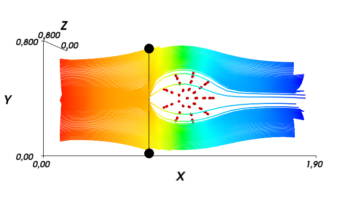
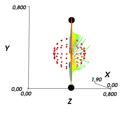
For a snack, a few pictures with a wrap around a sphere with a fairly high viscosity (and on a rather coarse grid).

Source: https://habr.com/ru/post/210276/

All Articles

Immersed boundary method for teapots

More articles: