Kalman, Matlab, and State Space Models
Kuznetsovin recently published a post about using Python to analyze time series in the economy. As a model, the "workhorse" of econometrics was chosen - ARIMA, perhaps, one of the most common models for time data. At the same time, the main disadvantage of ARIMA-like models is that they are not adapted for working with non-stationary rows. For example, if there is a trend or seasonality in the data, the expectation will have a different meaning in different parts of the series - 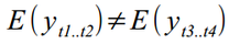 that is not good. To avoid this, ARIMA expects to work not with the original data, but with their difference (the so-called differentiation - from “taking a difference”). Everything would be fine, but two problems arise here - (a) we may lose significant information by taking the difference of a series, and (b) the opportunity to decompose a series of data into its constituent components — trend, cycle, etc. — is missed. Therefore, in this article I would like to give an alternative method of analysis - State Space Modeling (SSM), in Russian translation - the State Space Model.
So let's get started.
This part is one of the most important parts of the process, because if you make a mistake now, then the rest of the work may simply be a waste of time. We open the data on the shipment of goods at one of the warehouse complexes in the Moscow region, which were used in the previous article. Build a graph:
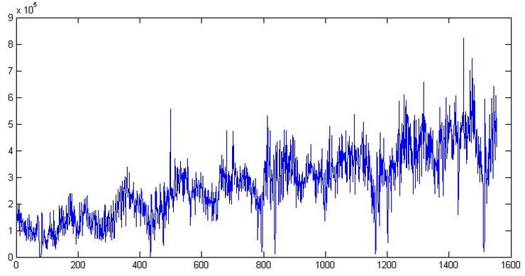
First, there is clearly a trend and cycle with an order of about 300 days. Now close the chart. Let's go smoke. We will come, we will open it again and look at the numbers themselves. The date of shipment is in format 01.09.2009, so we open it in Excel and if we translate the data into the format [$ -F800] dddd, mmmm dd, yyyy] so that the day of the week is shown, we note that usually on Saturday the shipping values are much lower than the rest of the week. For example, two weeks are shown in Graph 1. In general, the loader Uncle Vasya goes home on Saturday to watch football early, and because of this, we will have to take into account the presence of a microcycle with a seasonality of 7 days. By the way, we will not translate the data into a weekly interval, as in the previous article, but continue to work with daily data.
')
Here I will try to give a minimum of theory, more detailed why and where all the formulas come from can be found in the book or I will answer in the comments.
Suppose there is a certain time series In our case - the data on the shipment of goods. As kuznetsovin correctly pointed out in the previous article, the data are clearly non-stationary next to the integration order of 1, and the ARIMA procedure would require differentiation of the series. But since we do not want to do this, then following Harvey [1993], let us assume that this series can be represented as a model with unobservable components (Unobservable Component model):

Where - the observed series at time t , which consists of unobservable components: the trend  cycle
cycle  seasonal variable
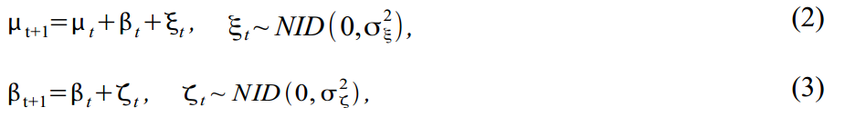
  (in our case equal to one week), and errors
  which is normally distributed as white noise
 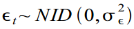 .
.
You can diversify a trend by building it as a model of a local linear trend:
where (2) is the actual trend and (3) is the slope of the trend, each with its own mistakes. This model provides many options for modeling the trend, from random walk with drift to the integrated random walk model. Many econometricians often remove an error in (2) to get a smooth, smooth trend, and assign random inclination to all random errors.
The stochastic cycle is modeled as the sum of trigonometric functions and their derivatives:
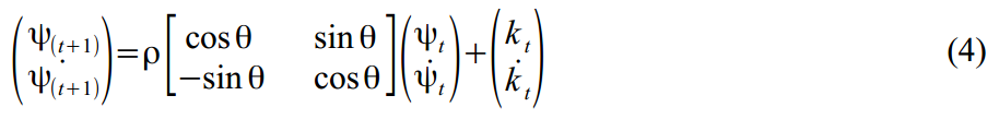
Where denotes the frequency of the cycle, which is measured in radians
 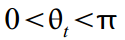 with the cycle period respectively
  . If there is a mood and extra time, we can assume that the frequency changes with time:
  but we will close our eyes and assume that the cycle is completely stationary. The attenuation coefficient is responsible for ensuring that our cycle does not fly beyond reasonable limits:
 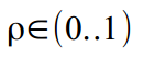 .
.
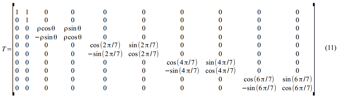
And finally, a weekly microcycle with a period of s = 7 will also be built on the basis of the sum of trigonometric functions:

Now all the above formulas are left organized in a so-called structural format suitable for the Kalman filter:
The measurement equation describes the data we observe:

and the transition equation - describes the dynamics of the variables that make up , but we do not see them (the so-called unobserved or latent variables):

In our case, there are 10 latent variables that were defined in equations (2) - (6):

Now we will translate all the above formulas into a matrix format.
Transition matrix in (7):

A weak matrix of the dynamics of latent variables in (8):
The vector of all errors of all states (2) - (6):

which is embedded in the equations of dynamics (8) using a matrix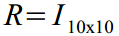 .
.
And finally, the matrix of variations of all errors and perturbations in (8):
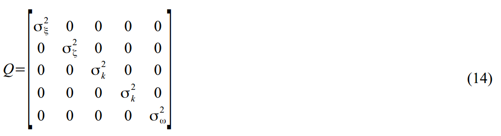
Ok, now we are ready to smoke Kalman. The filter algorithm has already been repeatedly written , except that we have slightly changed thenames and surnames of variable designations. Therefore, we will not dwell on the theory, only briefly for about forty minutes. So, there is a visible variable and a set of invisible  , for which we invented the dynamics and structure in (8) - (14), and which we try to calculate
 in parrots using the Kalman filter. Since the latent states are invisible, the model may not be particularly true, and various measurement errors are sure to occur, we are unlikely to meet, and only its expectation at time t based on the observed data 1, .., t-1 : 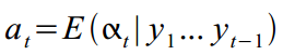 which has a variance
  .
.
Suppose the initial values known (in the practical part of the implementation of the algorithm, we simply specify values from the ceiling), the Kalman filter consists of a set of iterations:
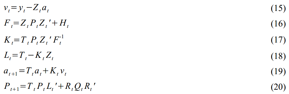
Where - one-time forecast error with variation
  ,
,  - Kalman gain, and so on. In general, the theory in Africa is the same - that in physics, that in geolocation. Only the variable notation is changed at the request of the author.
In addition to calculating the state vector, we are also interested in finding individual model parameters, such as error variation, cycle frequency, and cycle attenuation parameter. Call the vector of the required parameters as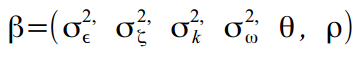 . Then if
  and
and  distributed according to Gauss, then the logarithmic likelihood function (Log-likelihood function) of the parameters for our data will be:

Because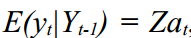 and
and  then the result from the Kalman filter can be used to calculate the likelihood function based on filter errors:

By maximizing this function, we can find estimates of the required parameters. . In practice, it is always easier to minimize functions, so we added minus signs in (22), and we will minimize it.
Now a few words about another wunderwaffe - Kalman Smoothing (Kalman smoother), [Durbin, J., and Koopman, 2003], which has not yet been mentioned in Habré. In general, the idea is similar, only the Kalman filter calculates each subsequent value. at time t based on previous data 1..t-1 :
 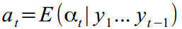 . And Kalman Smoother reads a little, and, assuming that we already have all the data, makes it possible to clarify looking at the whole time series
  that is, in simple words, it computes
  . This works well when we already have all the observations and are not interested in future estimates, but rather
 it is better to dress the exact values of the latent variables that make up the dynamics of the series.
Kalman smoothing is a reverse recursion:
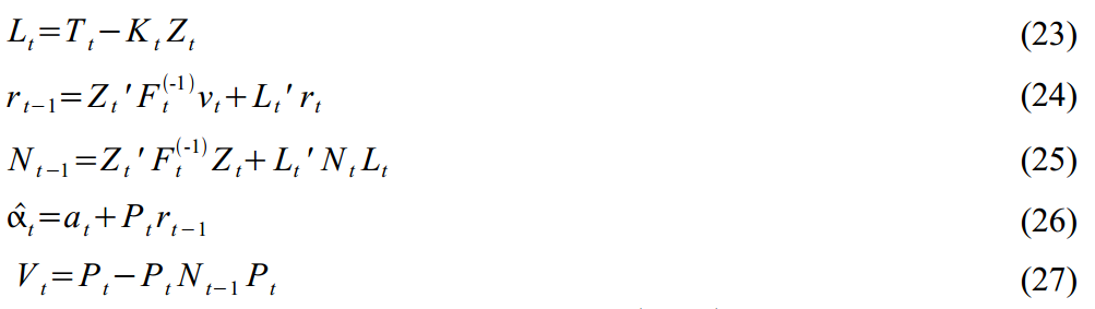
where is the smooth state vector will have the smallest variance  . Smoothing recursion begins at time t = N , and is started backwards, setting zero values to the vector
  and its dispersions
  . Forecast error values
  its dispersion and Kalman gain taken from the filter, which is driven in the first run.
In general, you can still write about the theory for a long time, but already itching to test. So, let's move on to empirical materialism.
I do not pretend to the optimality and speed of the following programs in Matlab, I am not a real welder, all the code was written for myself. Unaesthetic, but cheap, reliable and practical. Also, the code for the filter and the smoother is somewhat redundant, since it is written for different initialization variants and so on. Attempting to throw out part of the code inevitably led to Matlab's departures getting lost in the matrices and cycles, and so I decided to leave everything as it is.
Everything works like this:
Actually, the code:
(p-values of the found estimates are shown in brackets)
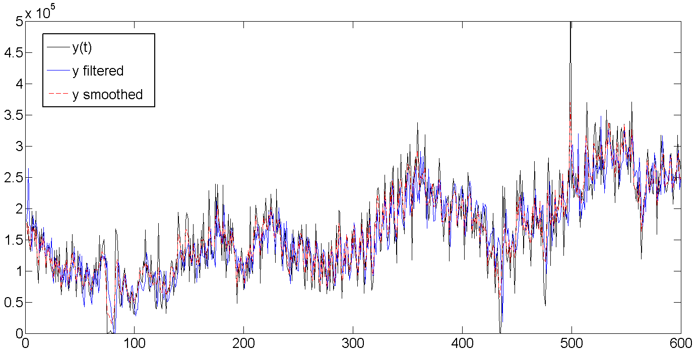
For convenience of perception, the graphs are shown only for the first 600 days, hidden for spoilers for the whole series.
a. Original, filtered, and smoothed data
b. Baseline, filtered trend, smoothed trend
As you can see, the Kalman filter tries to guess the trend based on previous values, and therefore oscillates along with the batch line, but is a bit late, trying to guess where our data will go further. The Kalman smoother “sees” the entire series, and therefore the trend looks much smoother and calmer:

c. Filtered and smoothed cycle
As can be seen from the table with the results, the average cycle length is about 362 days, or almost one year (who would be surprised). It also shows how at the very beginning the filter begins to be calibrated and completely misses the data, because we set the initial values of the latent variables to zero and a very large variance of about 1e + 10. But usually a few (2-5) first attempts are enough to filter the rhythm. By the way, exact initialization of the filter (exact initialization) was used in this work, which helps the filtered values to run faster with the data.

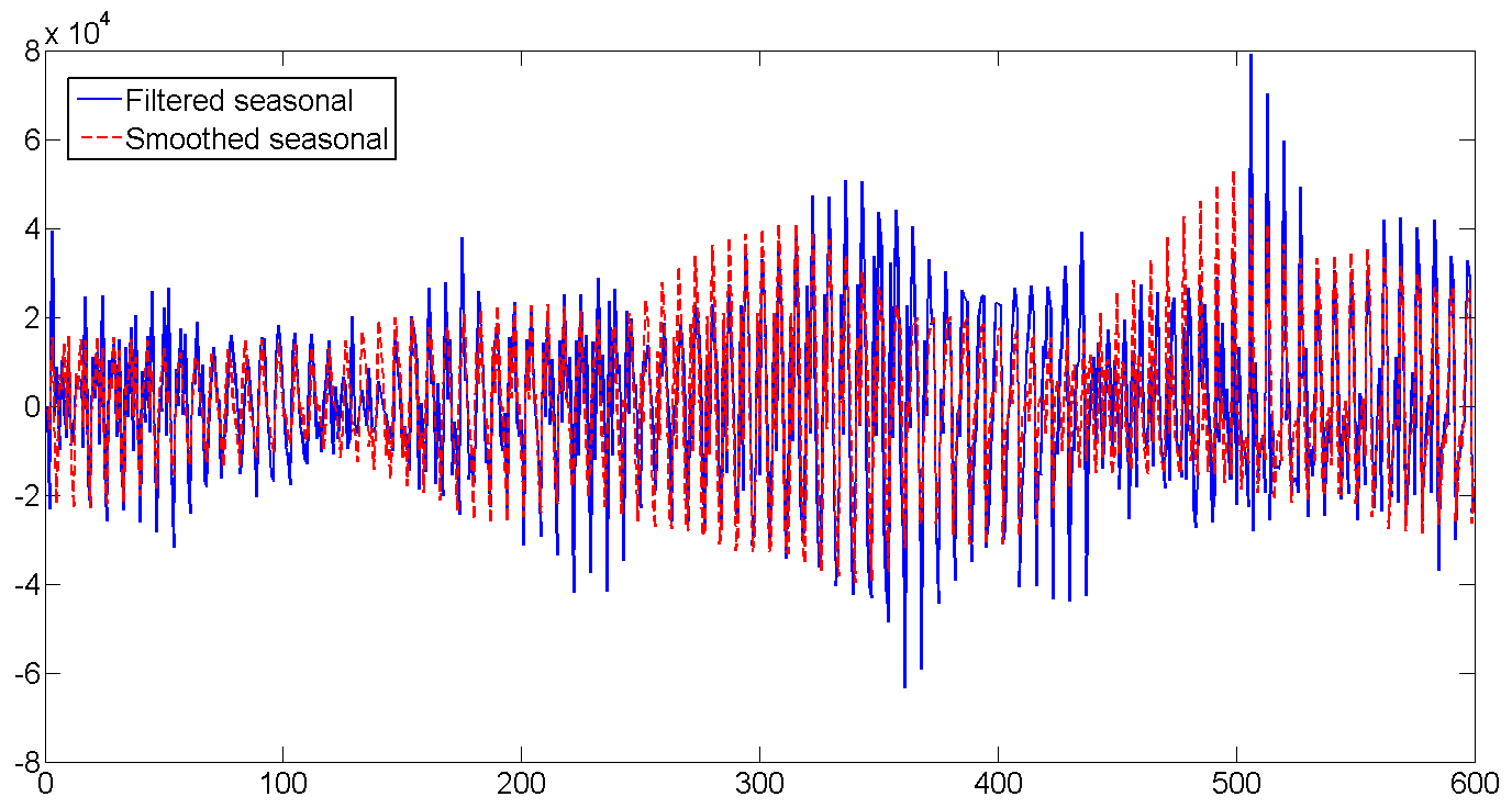
d. Filtered and smoothed weekly seasonal factor
The number of shipments is gradually increasing, and the daily volatility increases:
Based on the obtained parameters and using the latest values of the filtered states, we build a forecast for 70 days (10 weeks) and compare it with the existing data. In general, the forecast looks good, that's what the life-giving filter does. Especially pleased guessed volatility on days of the week. If you look at the entire length of the forecast and turn on the imagination, you can also see how the forecast bends under the annual cycle of shipment. The only time where the forecast did not work - from 26 to 32 days. But there was clearly an almost weekly drop in shipments, as well as a sharp jump immediately behind it, which it was hardly possible to foresee, since such a case occurred only once at the very beginning of the series. In general, and what fell, so from cloudiness.
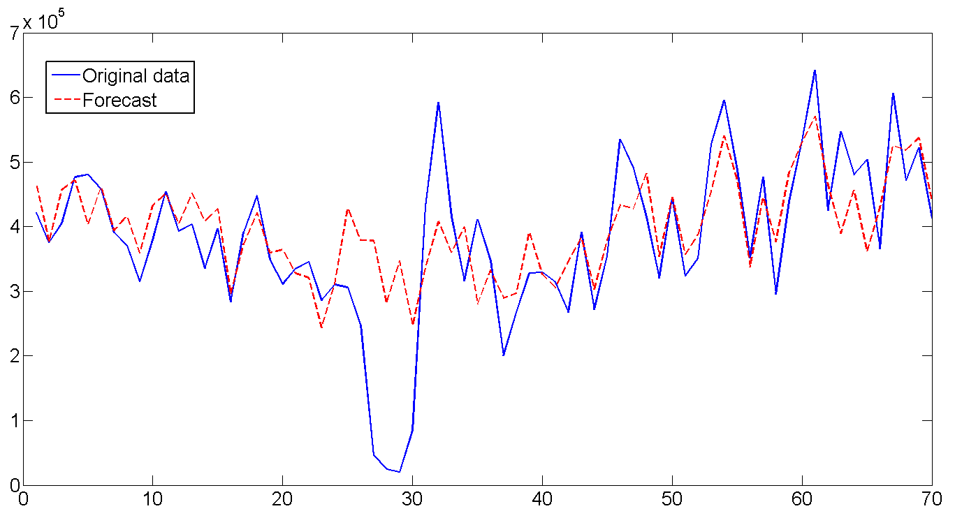
The forecast RMSE is 1.112e + 005, in case we want to compare the model.
Well that's all.
Note
For many English-language names in this area, the translation is either absent or different from different translators, or clumsy until it is completely impossible to use it in a decent society. Therefore, many names will be given in the English version. For those interested - one of the best books on SSM modeling. It also turned out that in the Russian-language translation there are practically no good books on the topic. As an option - the work of Alexander Tsyplakov, which, although published as a separate article, is actually a copy of the book in an extremely abridged version.
So let's get started.
1. Initial data analysis
This part is one of the most important parts of the process, because if you make a mistake now, then the rest of the work may simply be a waste of time. We open the data on the shipment of goods at one of the warehouse complexes in the Moscow region, which were used in the previous article. Build a graph:
First, there is clearly a trend and cycle with an order of about 300 days. Now close the chart. Let's go smoke. We will come, we will open it again and look at the numbers themselves. The date of shipment is in format 01.09.2009, so we open it in Excel and if we translate the data into the format [$ -F800] dddd, mmmm dd, yyyy] so that the day of the week is shown, we note that usually on Saturday the shipping values are much lower than the rest of the week. For example, two weeks are shown in Graph 1. In general, the loader Uncle Vasya goes home on Saturday to watch football early, and because of this, we will have to take into account the presence of a microcycle with a seasonality of 7 days. By the way, we will not translate the data into a weekly interval, as in the previous article, but continue to work with daily data.
')
Chart 1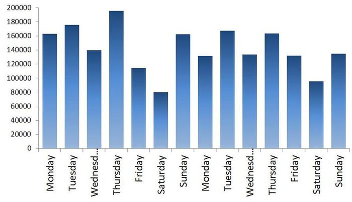
2. State Space Modes
Here I will try to give a minimum of theory, more detailed why and where all the formulas come from can be found in the book or I will answer in the comments.
Suppose there is a certain time series
Where
You can diversify a trend by building it as a model of a local linear trend:
where (2) is the actual trend and (3) is the slope of the trend, each with its own mistakes. This model provides many options for modeling the trend, from random walk with drift to the integrated random walk model. Many econometricians often remove an error in (2) to get a smooth, smooth trend, and assign random inclination to all random errors.
The stochastic cycle is modeled as the sum of trigonometric functions and their derivatives:
Where
And finally, a weekly microcycle with a period of s = 7 will also be built on the basis of the sum of trigonometric functions:
Now all the above formulas are left organized in a so-called structural format suitable for the Kalman filter:
The measurement equation describes the data we observe:
and the transition equation - describes the dynamics of the variables that make up
In our case, there are 10 latent variables that were defined in equations (2) - (6):
Now we will translate all the above formulas into a matrix format.
Transition matrix in (7):
A weak matrix of the dynamics of latent variables in (8):
The vector of all errors of all states (2) - (6):
which is embedded in the equations of dynamics (8) using a matrix
And finally, the matrix of variations of all errors and perturbations in (8):
3. Filter and Kalman Smoother
Ok, now we are ready to smoke Kalman. The filter algorithm has already been repeatedly written , except that we have slightly changed the
Suppose the initial values
Where
In addition to calculating the state vector, we are also interested in finding individual model parameters, such as error variation, cycle frequency, and cycle attenuation parameter. Call the vector of the required parameters as
Because
By maximizing this function, we can find estimates of the required parameters.
Now a few words about another wunderwaffe - Kalman Smoothing (Kalman smoother), [Durbin, J., and Koopman, 2003], which has not yet been mentioned in Habré. In general, the idea is similar, only the Kalman filter calculates each subsequent value.
Kalman smoothing is a reverse recursion:
where is the smooth state vector
In general, you can still write about the theory for a long time, but already itching to test. So, let's move on to empirical materialism.
4. Regression
I do not pretend to the optimality and speed of the following programs in Matlab, I am not a real welder, all the code was written for myself. Unaesthetic, but cheap, reliable and practical. Also, the code for the filter and the smoother is somewhat redundant, since it is written for different initialization variants and so on. Attempting to throw out part of the code inevitably led to Matlab's departures getting lost in the matrices and cycles, and so I decided to leave everything as it is.
Everything works like this:
- The main program otgr_ssm.m loads data, prepares the ssmopt structure, which contains many valuable comments and important variables that will be transmitted to different places in the code. The last 70 values for shipment (10 weeks) will be set aside for comparison with the forecast, which we will definitely build at the end.
- The data is uploaded to the maximization routine Log-likelihood function. The latter procedure is often used in econometrics, so it was quickly written on the knee in general form as a separate function mle_my.m so as not to litter the main code.
- since the desired parameters include the dispersions of states, they must be strictly positive, which is not always obtained in the course of numerical optimization. Therefore, we change pawns to ryumash and all input values of the variances will be transformed as
 and the value of the attenuation coefficient is normalized in the range
  as
as  . Well, at the output, it is transformed back to get the correct values -
  for variations and
  for attenuation coefficient. The ssmopt.trans value indicates whether to transform (1) or not (0), and which way is 'in', or 'out'. All this happens with the help of a separate function transform.m
 - mle_my.m calls the object function f_obj.m , which runs the Kalman filter (15) - (22) using kfmy2.m , calculates the value of the Log-likelihood function (22), and, in order not to get up, calculates the Kalman Smoother (23 ) - (27) using ksmy2.m . This is all sent back to mle_my.m , which checks whether we have reached the maximum of function (22) or not. If yes, then everything is on the way out, to point 5. If not, then repeat steps 2-4.
The very first start of the filter begins with the assumption that . Here you can play, because there are a lot of variables, and we are searching for the global maximum of the six-dimensional function, therefore many local extremes are possible. In an amicable way, one could construct graphs of possible values of the log function and look at possible extremes.
 - We display the results - found parameters and graphs. At the same time let's calculate the prediction for 70 days and compare it with real data using frcst.m
Actually, the code:
otgr_ssm.m
clear all; clc; close all; format long; %------------------- 1. Load and prepare data ------------------------------ load otgruzka.mat; % Structure ssmopt contains several important records used throughout the code ssmopt.frcst=70; % forecast length yend=y(end-ssmopt.frcst+1:end); % saved last observation for the forecast comparison y=y(1:end-ssmopt.frcst); ssmopt.N=length(y); ssmopt.trans=1; % transform estimated parameters to preserve positiveness of variances ssmopt.sv=[5e+8;500;5e+8;5e+8;0.05;0.9]; % starting values ssmopt.mle='f_obj'; % name of the objective function for the maximization ssmopt.sv=transform(ssmopt.sv,'in',ssmopt); ssmopt.filter='kfmy2'; % name of the function computing Kalman Filter ssmopt.smooth='ksmy2'; % name of the function computing Kalman Smoother %------------------- 2. Estimate the model ------------------------------ result=mle_my(y,ssmopt); % call Maximum Likelihood maximization function b=transform(result.b,'out',ssmopt); % transform parameters back % recompute data based on the correct non-transformed parameters ssmopt.trans=0; ssmopt.sv=b; [LH,KF_out,Ksm_out] = feval(ssmopt.mle,b,y, ssmopt); % Recover filtered states series - trend, cycle, and seasonal a_trend=KF_out.Afilt(1,:); a_cycle=KF_out.Afilt(3,:); a_seas=KF_out.Afilt(5,:)+KF_out.Afilt(7,:)+KF_out.Afilt(9,:); y_filt=a_trend+a_cycle+a_seas; % build the estimated filtered series Y % Recover smoothed states series - trend, cycle, and seasonal a_trendsm=Ksm_out.Asm(1,:); a_cyclesm=Ksm_out.Asm(3,:); a_seassm=Ksm_out.Asm(5,:)+Ksm_out.Asm(7,:)+Ksm_out.Asm(9,:); y_smooth=a_trendsm+a_cyclesm+a_seassm; % build the estimated smoothed series Y result=mle_my(y,ssmopt); % find correct Hessian for non-transformed parameters %------------------- 3. Compute estimation statistics ------------------------------ %Find standard errors, and p-values se=sqrt(abs(diag(inv(result.hessian)/ssmopt.N))); % se(b) tstat=b./se; % t-statistics pval=2*(1-tcdf(abs(tstat),ssmopt.N-length(ssmopt.sv))); % p-value % Display output fprintf('Estimated parameters and p-values:\n'); out=[b pval] period=2*pi/b(end-1) % Compute R-squared resid=y-y_filt; % estimation errors SSE=resid*resid'; % Sum of Squared Errors SST=(y-mean(y))*(y-mean(y))'; % Sum of Squares Total R2=1-SSE/SST % R-squared' %------------------- 4. Make Forecast ------------------------------ af0=KF_out.Afilt(:,end-ssmopt.frcst); [yf,af]=frcst(b,y,ssmopt, af0); %------------------- 5. Plot results ------------------------------ %p=ssmopt.N; p=600; t=[1:1:p]; figure(1) plot(t,y(1:p),'k',t,y_filt(1:p),'b',t,y_smooth(1:p),'r--') title('Original, Filtered, and Smoothed data') legend('y(t)','y filtered','y smoothed'); figure(2) plot(t,y(1:p),'k',t,a_trend(1:p),'b',t,a_trendsm(1:p),'r--') title('Original data, Filtered and Smoothed trend') legend('y(t)','Filtered trend','Smoothed trend'); figure(3) plot(t,a_cycle(1:p),'b',t,a_cyclesm(1:p),'r--') title('Filtered and Smoothed cycle') legend('Filtered cycle','Smoothed cycle'); figure(4) % Filtered + smoothed seasonal plot(t,a_seas(1:p),'b',t,a_seassm(1:p),'r--') title('Filtered and Smoothed weekly seasonal') legend('Filtered seasonal','Smoothed seasonal'); t=[1:1:ssmopt.frcst]; figure(5) plot(t,yend,'b',t,yf,'r--') title('Original data and Forecast') legend('Original data','Forecast'); RMSE=sqrt(sum((yend - yf).^2)/ssmopt.frcst) % Root Mean Squared Error mle_my.m
function result_mle=mle_my(y,mleopt); warning off; %---------------- 1. Set-up minimization options ---------------- options=optimset('fminunc'); options=optimset('LargeScale', 'off' , ... 'HessUpdate', 'bfgs' , ... 'LineSearchType', 'quadcubic' , ... 'GradObj' , 'off' , ... 'Display','off' , ... 'MaxIter' , 1000 , ... 'TolX', 1e-12 , ... 'TolFun' , 1e-12, ... 'DerivativeCheck' , 'off' , ... 'Diagnostics' , 'off' , ... 'MaxFunEvals', 1000); %---------------- 2. Run minimization ---------------- [b,fval,exitflag,output,grad,hessian]=fminunc(mleopt.mle,mleopt.sv,options,y,mleopt); warning on; result_mle.b=b; result_mle.fval=fval; result_mle.output=output; result_mle.hessian=hessian; f_obj.m
function [obj,KF_out,Ksm_out]=f_obj_tr(b,y,ssmopt); %---------------- 1. Recover parameters ------------------------------------ b=transform(b,'out',ssmopt); s2_irr=b(1); s2_tr=b(2); s2_cyc=b(3); s2_seas=b(4); freq=b(5); rho=b(6); %---------------- 2. Build the model ------------------------------------ ssmopt.ssmodel.states=10; ssmopt.ssmodel.Z=[1 0 1 0 1 0 1 0 1 0]; T1 = [1 1 0 0; 0 1 0 0; 0 0 rho*cos(freq) rho*sin(freq); 0 0 -rho*sin(freq) rho*cos(freq)]; T2=[cos(2*pi/7) sin(2*pi/7) 0 0 0 0;... -sin(2*pi/7) cos(2*pi/7) 0 0 0 0;... 0 0 cos(4*pi/7) sin(4*pi/7) 0 0;... 0 0 -sin(4*pi/7) cos(4*pi/7) 0 0;... 0 0 0 0 cos(6*pi/7) sin(6*pi/7);... 0 0 0 0 -sin(6*pi/7) cos(6*pi/7)]; ssmopt.ssmodel.T = [T1 zeros(rows(T1),cols(T2));zeros(rows(T2),cols(T1)) T2]; ssmopt.ssmodel.R=eye(10); ssmopt.ssmodel.R(1,1)=0; H=s2_irr; Q=zeros(10,10); Q(2,2)=s2_tr; Q(3,3)=s2_cyc; Q(4,4)=s2_cyc; Q(5,5)=s2_seas; Q(6,6)=s2_seas; Q(7,7)=s2_seas; Q(8,8)=s2_seas; Q(9,9)=s2_seas; Q(10,10)=s2_seas; %---------------- 3. Suggest starting conditions for the states ------------------------ a0=[y(1);0;0;0;0;0;0;0;0;0]; P0=eye(ssmopt.ssmodel.states)*1e+10; %---------------- 4. Run Kalman filter ------------------------ KF_out = feval(ssmopt.filter,y, ssmopt, Q, H, a0, P0); obj=KF_out.LH; %---------------- 5. Run Kalman smoother ------------------------ if nargout>2 ssmopt.ssmodel.num_etas=3; % number of the state variances (required for Kalman smoother) Ksm_out = feval(ssmopt.smooth,KF_out, ssmopt); end kfmy2.m
% Kalman filter % y[t] = Z*alpha[t] + eps, eps ~ N(0,H). % alpha[t] = T*alpha[t-1] + R*eta, eta ~ N(0,Q). % v[t]=y[t]-E(y[t]) = y[t]-Z*a[t] % F[t]=var(v[t]) function KF_out = kfmy_koop(y, ssmopt, Q, H, a, P); N=ssmopt.N; m=ssmopt.ssmodel.states; %---------------- 1. Recover parameters and prepare matrices ---------------- T=ssmopt.ssmodel.T; Z=ssmopt.ssmodel.Z; R=ssmopt.ssmodel.R; KF_out.Vmat=zeros(1,N); KF_out.Fmat=zeros(1,N); KF_out.Afilt=zeros(m,N); KF_out.Pfilt=zeros(m,m,N); KF_out.Kmat=zeros(m,N); KF_out.Lmat=zeros(m,m,N); LHmat=zeros(1,N); if ~isfield(ssmopt,'exactcheck'); ssmopt.exactcheck=1; % set exact filter initialization by default end; %---------------- 2. Set default starting values for a and P , if none provided ---------------- Pinf=eye(m); if nargin < 6 if ssmopt.exactcheck==1 P=zeros(m,m); else P=eye(m)*1000000000; end end if nargin < 5 a=[y(1); zeros(m-1,1)]; end KF_out.Afilt(:,1)= a; KF_out.Pfilt(:,:,1) = P; d=0; %---------------- 3. Exact Filtering ---------------- if ssmopt.exactcheck==1 evals=10; % number of time steps to evaluate until Pinf converges to zero KF_out.exact.F1=zeros(1,evals); KF_out.exact.F2=zeros(1,evals); KF_out.exact.L1=zeros(m,m,evals); KF_out.exact.Pinf=zeros(m,m,evals); KF_out.exact.Pinf(:,:,1)=Pinf; for i=1:evals if sum(sum(Pinf))<1e-20; d=i-1; % time point after which Pinf-->0, and after which we may start regular Kalman filter break; else if sum(Pinf*Z')>0 % Pinf is not singular F1=inv(Z*Pinf*Z'); F2=-F1*(Z*P*Z'+H)*F1; K=T*Pinf*Z'*F1; K1=T*(P*Z'*F1+Pinf*Z'*F2); L=TK*Z; L1=-K1*Z; P=T*Pinf*L1' + T*P*L' + R*Q*R'; Pinf=T*Pinf*L'; else F1=Z*P*Z'+H; F2=F1; K=T*P*Z'/F1; L=TK*Z; L1=L; P=T*P*L' + R*Q*R'; Pinf=T*Pinf*T'; end v=y(i) - Z*a; a=T*a+K*v; %save filtered estimates KF_out.Afilt(:,i+1)=a; KF_out.Pfilt(:,:,i+1)=P; KF_out.Vmat(i)=v; KF_out.Fmat(i)=F1; KF_out.Kmat(:,i)=K; KF_out.Lmat(:,:,i)=L; LHmat(i) = -0.5*(log(2*pi*F1) + v^2/F1); %save exact values for smoother KF_out.exact.F1(i)=F1; KF_out.exact.F2(i)=F2; KF_out.exact.L1(:,:,i)=L1; KF_out.exact.Pinf(:,:,i+1)=Pinf; end end end %---------------- 4. Regular Filtering ---------------- for i=d+1:N v=y(i) - Z*a; f=Z*P*Z' + H; K=T*P*Z'/f; L=TK*Z; a=T*a+K*v; P=T*P*L'+R*Q*R'; if i<N KF_out.Afilt(:,i+1)=a; KF_out.Pfilt(:,:,i+1)=P; end KF_out.Vmat(i)=v; KF_out.Fmat(i)=f; KF_out.Kmat(:,i)=K; KF_out.Lmat(:,:,i)=L; LHmat(i) = -0.5*(log(2*pi*f) + v^2/f); end %---------------- 5. Prepare output ---------------- KF_out.LH=-sum(LHmat); KF_out.Q=Q; KF_out.H=H; KF_out.exact.d=d; end ksmy2.m
function [Ksm_out, Kdism_out] = ksmy2(KF_out, ssmopt); [m,N]=size(KF_out.Afilt); meta=ssmopt.ssmodel.num_etas; %---------------- 1. Recover filtered matrices ---------------- Fmat=KF_out.Fmat; Vmat=KF_out.Vmat; Pfilt=KF_out.Pfilt; Afilt=KF_out.Afilt; Q=KF_out.Q; H=KF_out.H; %---------------- 2. Recover Model structure ---------------- Z=ssmopt.ssmodel.Z; T=ssmopt.ssmodel.T; R=ssmopt.ssmodel.R; Asm=zeros(m,N); Psm=zeros(m,m,N); rmat=zeros(m,N); Nmat=zeros(m,m,N); Eps=zeros(1,N); Eta=zeros(meta,N); Kmat=KF_out.Kmat; Lmat=KF_out.Lmat; if ~isfield(KF_out,'exact'); KF_out.exact.d=0; end d=KF_out.exact.d; if KF_out.exact.d>0 L1=KF_out.exact.L1; F1=KF_out.exact.F1; F2=KF_out.exact.F2; Pinf=KF_out.exact.Pinf; end %---------------- 3. Regular Smoothing for t=N..d+1 observations ---------------- for i=N:-1:d+1 r=Z'/Fmat(i)*Vmat(i) + Lmat(:,:,i)'*rmat(:,i); N=Z'/Fmat(i)*Z + Lmat(:,:,i)'*Nmat(:,:,i)*Lmat(:,:,i); Asm(:,i)=Afilt(:,i) + Pfilt(:,:,i)*r; Psm(:,:,i)=Pfilt(:,:,i)-Pfilt(:,:,i)*N*Pfilt(:,:,i); if i>1 rmat(:,i-1)=r; Nmat(:,:,i-1)=N; end if nargout>1 Eps(i)=H*(1/(Fmat(i))*Vmat(i)-Kmat(:,i)'*rmat(:,i)); Eta(:,i)=Q*R'*rmat(:,i); end end %---------------- 4. Exact Smoothing for t=d..1 observations ---------------- if KF_out.exact.d>0 r1=zeros(m,1); N1=zeros(m,m); N2=zeros(m,m); for i=d:-1:1 if sum(Pinf(:,:,i)*Z')>0 %cond(Pinf)<1e+12 % Pinf is not singular r1=Z'*F1(i)*Vmat(i) + Lmat(:,:,i)'*r1 + L1(:,:,i)'*rmat(:,i); N2=Z'*F2(i)*Z + Lmat(:,:,i)'*N2*Lmat(:,:,i) + Lmat(:,:,i)'*N1*L1(:,:,i) + L1(:,:,i)'*N1*Lmat(:,:,i) + L1(:,:,i)'*Nmat(:,:,i)*L1(:,:,i); N1=Z'*F1(i)*Z + Lmat(:,:,i)'*N1*Lmat(:,:,i) + L1(:,:,i)'*Nmat(:,:,i)*Lmat(:,:,i); r=Lmat(:,:,i)'*r1; N=Lmat(:,:,i)'*Nmat(:,:,i)*Lmat(:,:,i); if nargout>1 Eps(i)=-H*Kmat(:,i)'*rmat(:,i); Eta(:,i)=Q*R'*rmat(:,i); end else % Pinf is singular r1=T'*rmat(:,i); N2=T'*N2*T; N1=T'*N1*Lmat(:,:,i); r=Z'/(Fmat(i))*Vmat(i) + Lmat(:,:,i)'*rmat(:,i); N=Z'/(Fmat(i))*Z + Lmat(:,:,i)'*Nmat(:,:,i)*Lmat(:,:,i); if nargout>1 Eps(i)=H*(1/Fmat(i)*Vmat(i) - Kmat(:,i)'*rmat(:,i)); Eta(:,i)=Q*R'*rmat(:,i); end end if i>1 rmat(:,i-1)=r; Nmat(:,:,i-1)=N; end Asm(:,i)=Afilt(:,i) + Pfilt(:,:,i)*r + Pinf(:,:,i)*r1; Psm(:,:,i)=Pfilt(:,:,i)-Pfilt(:,:,i)*N*Pfilt(:,:,i) - (Pinf(:,:,i)*N1*Pfilt(:,:,i))' - Pinf(:,:,i)*N1*Pfilt(:,:,i) - Pinf(:,:,i)*N2*Pinf(:,:,i); end end %---------------- 5. Prepare output ---------------- Ksm_out.Asm=Asm; Ksm_out.Psm=Psm; Ksm_out.Kmat=Kmat; Ksm_out.Lmat=Lmat; Ksm_out.Nmat=Nmat; Ksm_out.rmat=rmat; Kdism_out.Eps=Eps; Kdism_out.Eta=Eta; transform.m
function b=transform(b,howto,ssmopt); k=length(b); if strcmp(howto,'in') % in-transformation if ssmopt.trans==0 % no transformation b=b; end; if ssmopt.trans==1 % transformation to preserve the positiveness of variances b(1:k-1,:)=log(b(1:k-1,:)); b(k)=log(1/b(k)-1); end; else % out-transformation if ssmopt.trans==0 % no transformation b=b; end; if ssmopt.trans==1 b(1:k-1,:)=exp(b(1:k-1,:)); b(k)=1/(1+exp(b(k))); end; end 5. Results
(p-values of the found estimates are shown in brackets)
| The variance of the error of the observed series | 1.77E + 009 (0.00) |
| Trend Error Dispersion | 348.73 (0.00) |
| Cycle variance | 6.07E + 008 (0.00) |
| Seasonal component error variance | 3.91E + 006 (0.00) |
| Cycle frequency | 3.91E + 006 (0.00) |
| Cycle period (days) | 362.6 (0.00) |
| Cycle attenuation coefficient | 0.891 (0.00) |
| R-squared regression | 0.78 |
6. Charts
For convenience of perception, the graphs are shown only for the first 600 days, hidden for spoilers for the whole series.
a. Original, filtered, and smoothed data
Whole row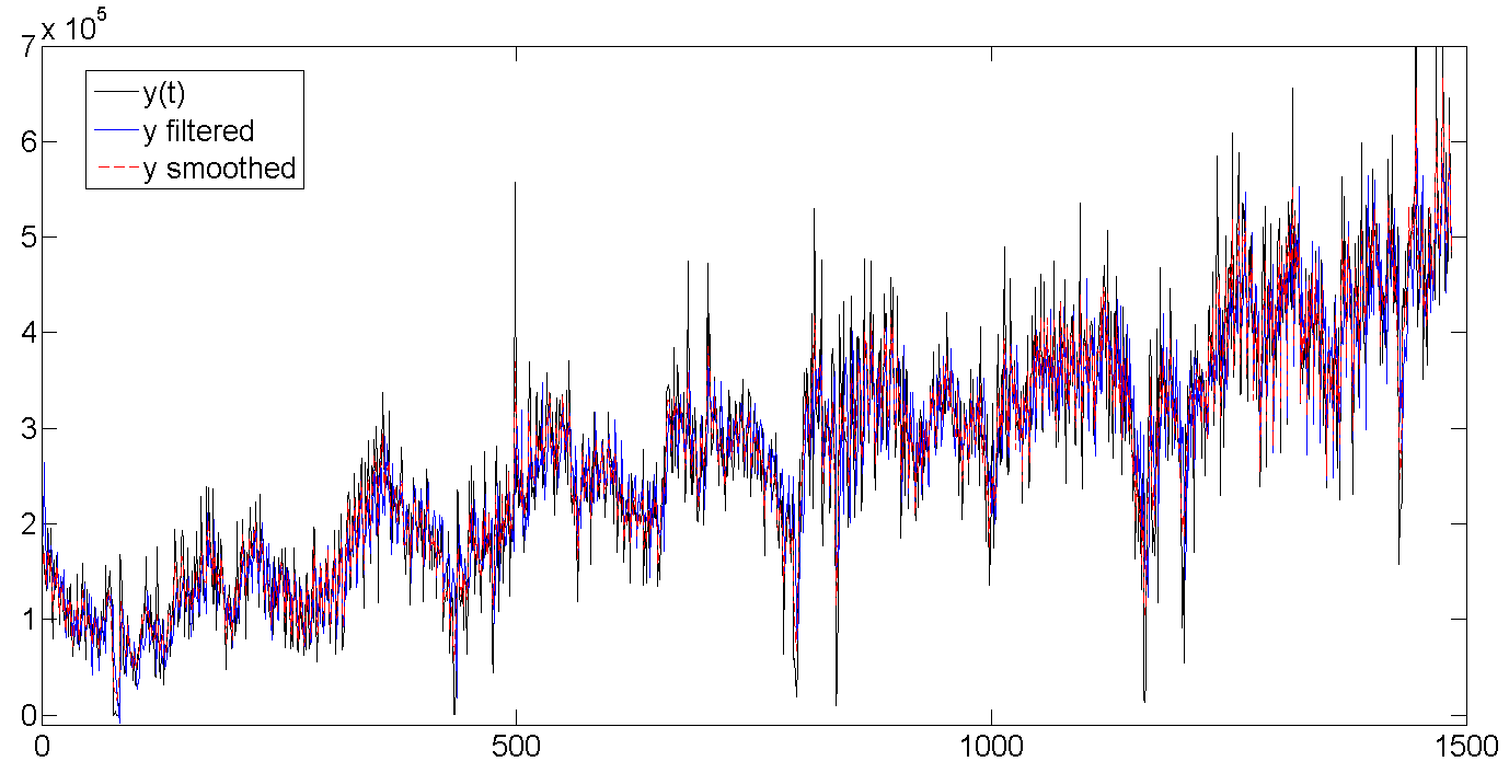
b. Baseline, filtered trend, smoothed trend
As you can see, the Kalman filter tries to guess the trend based on previous values, and therefore oscillates along with the batch line, but is a bit late, trying to guess where our data will go further. The Kalman smoother “sees” the entire series, and therefore the trend looks much smoother and calmer:
Whole row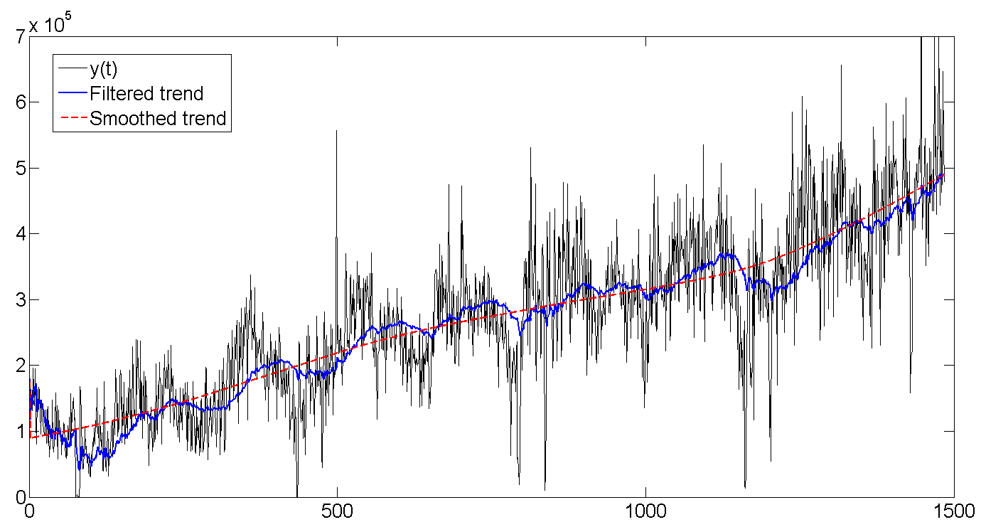
c. Filtered and smoothed cycle
As can be seen from the table with the results, the average cycle length is about 362 days, or almost one year (who would be surprised). It also shows how at the very beginning the filter begins to be calibrated and completely misses the data, because we set the initial values of the latent variables to zero and a very large variance of about 1e + 10. But usually a few (2-5) first attempts are enough to filter the rhythm. By the way, exact initialization of the filter (exact initialization) was used in this work, which helps the filtered values to run faster with the data.
Whole row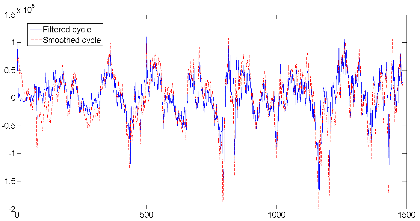
d. Filtered and smoothed weekly seasonal factor
The number of shipments is gradually increasing, and the daily volatility increases:
Whole row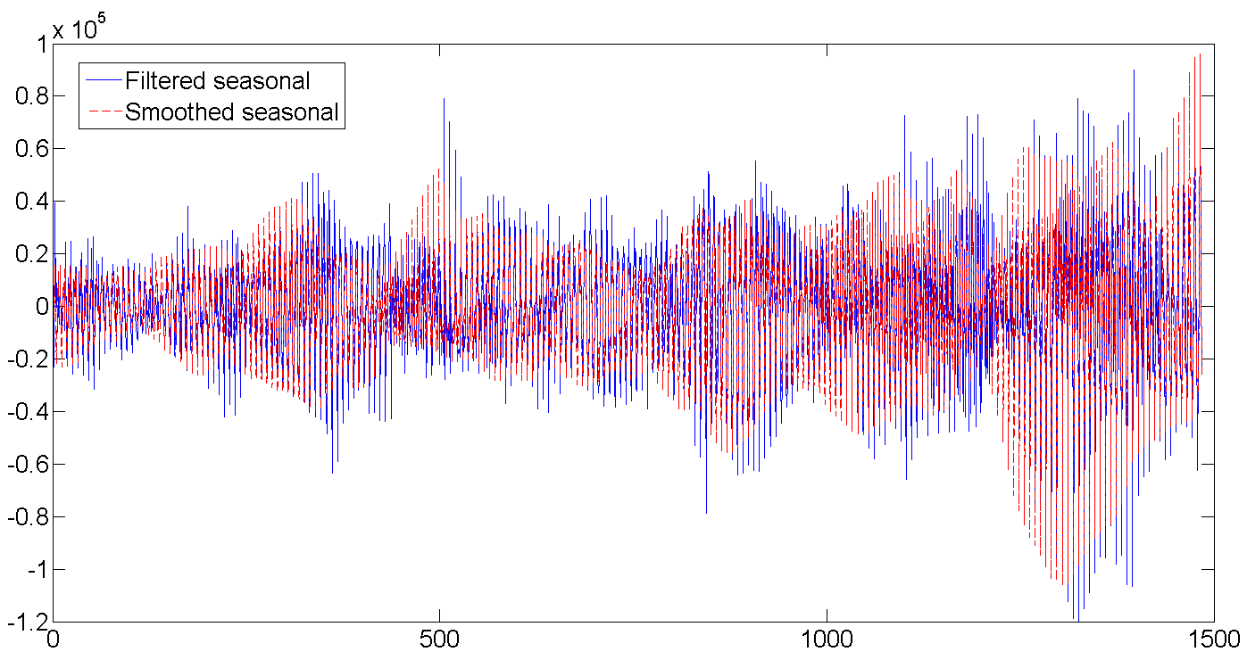
6. Forecast
Based on the obtained parameters and using the latest values of the filtered states, we build a forecast for 70 days (10 weeks) and compare it with the existing data. In general, the forecast looks good, that's what the life-giving filter does. Especially pleased guessed volatility on days of the week. If you look at the entire length of the forecast and turn on the imagination, you can also see how the forecast bends under the annual cycle of shipment. The only time where the forecast did not work - from 26 to 32 days. But there was clearly an almost weekly drop in shipments, as well as a sharp jump immediately behind it, which it was hardly possible to foresee, since such a case occurred only once at the very beginning of the series. In general, and what fell, so from cloudiness.
The forecast RMSE is 1.112e + 005, in case we want to compare the model.
Well that's all.
Note
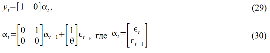
State Space Models should not be taken as something worthwhile in Econometrics. On the contrary, they represent a generic version for many more specific models. For example, MA (1) process

easy to imagine in SSM form:
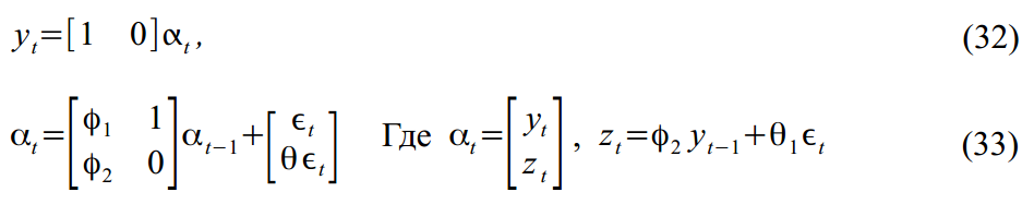
Or ARMA (2,1) process:

Packed in SSM format:
easy to imagine in SSM form:
Or ARMA (2,1) process:
Packed in SSM format:
Related Literature
- Durbin, J., and Koopman, SJ, Time Series Analysis by State Space Methods. Oxford: Oxford University Press, 2001.
- Durbin, J., and Koopman, SJ “A simple and efficient simulation for state space time analysis” Biometrika vol. 89, issue 3, 2002.
- Harvey, AC, and Jaeger, A. “Detrending, stylized facts and the business cycle.” Journal of Applied Econometrics (8), 1993.
- Harvey, AC Forecasting, Structural Time Series Models and the Kalman Filter. Cambridge: Cambridge University Press, 1989.
Source: https://habr.com/ru/post/209640/
All Articles