Introduction to optimization. Annealing imitation
In this article I will try to speak in the most intelligible way about such a simple but effective method of optimization as simulated annealing. And in order not to be numbered among those who are far from practice, those who like to theorize, I will show how to apply this method to solve the traveling salesman problem.
To understand the article, you will need minimal programming skills and mastery of mathematics at the grade 9 level of high school. The article is intended for people who are not familiar with optimization methods or who are just taking the first steps in this direction.

')
In order to maximize the circle of readers, I had to almost completely abandon formal definitions and consciously go for some not entirely accurate simplifications. I hope that with the water I did not throw out the child (and if this happened, I will be glad to your comments).
In order to understand what optimization is, you first need to know what it is for. At once I will say that with the “optimization problems” in everyday life we are confronted with enviable regularity, without giving ourselves a report on this.
Suppose we, having received the next salary, decide to line up the family budget. It is necessary to allocate money so that first of all to satisfy the most important needs (food, electricity, Internet, etc.), and the rest can be lowered to something lower priority. Buy all the money designer phone and die of hunger - not the best solution, is not it?
Or another option, we decided to go hiking and collect a satchel. One problem is that there is a lot of things, and our backpack is not too big (and we ourselves have limited carrying capacity). We want to take as many of the most important items for us as possible. If we go to the mountains, grabbing a safety cable with us is a good decision, take your favorite PlayStation Vita instead, and probably don’t give you the rest of the time with cookies.
So what does the optimization do? She is looking for the very good solution. Perhaps not the best of all, but definitely good.
Now a little bit more formal. If you look at Wikipedia, you can easily find the following definition:
The optimal (from the Latin. Optimus - the best) solution - a solution that, in one way or another, is preferable to others. Therefore, optimization is a way to find the optimal solution.
Now, let's imagine that we can measure how good our decision is. For example, in the case of a “knapsack problem”, we assign each thing a natural number (the larger the number, the more important the thing). Then our task gets a clearer statement: we want to fill the satchel with such things, the total priority of which will be maximum, and the weight will not exceed a certain value. Those. we are looking for the maximum of a certain function , which is called the target .
To reduce everything to a common denominator, look again at Wikipedia:
Optimization (mathematics) - finding the extremum (minimum or maximum) of the objective function in a certain area.
Now that we have more or less decided on what the optimization is doing, a reasonable question appears - “How?”.
Of course, we can not particularly bother and go through all the solutions, and then compare them. In the case of the knapsack, we can probably even do this. But now let's imagine that our satchel is not a satchel at all, but a whole train with many wagons, but we transport different goods to another city. The task has not changed (load as much as possible valuable), and the target function will be the total value of the goods. How long will it take us to complete a bust of solutions? I think a lot.
You can choose solutions randomly. Suppose there are a hundred solutions, and then take the best of them. Undoubtedly, it will be much faster than complete enumeration, but who will guarantee that our final solution will be at all close to the extremum?
I will not torment and say that there are a great many optimization methods . So much that they are usually divided into classes, I will not list them all. Let me just say that “annealing imitation” refers to the class of stochastic (from the Greek. Στχχσστικός - “ able to guess ”) or probabilistic methods. And where is the probability and how it will help find a solution - just below.
Like all brilliant, this method is peeped at Mother Nature. It is based on the process of crystallization of the substance, which in turn was “tamed” by sly metallurgists, in order to increase the homogeneity of the metal.
Let me remind you that every metal has a crystal lattice , if very briefly, it describes the geometric position of the atoms of matter. The set of positions of all atoms will be called the state of the system, each state corresponds to a certain level of energy. The purpose of annealing is to bring the system to the lowest energy state. The lower the energy level, the “better” the crystal lattice, i.e. the fewer defects and stronger the metal.
During the "annealing" the metal is first heated to a certain temperature, which causes the atoms of the crystal lattice to leave their positions. Then begins a slow and controlled cooling. Atoms tend to get into a state with less energy, however, with a certain probability they can go into a state with more. This probability decreases with temperature. The transition to the worst state, oddly enough, helps in the end to find a state with energy less than the initial one. The process ends when the temperature drops to a predetermined value.
As you can see, in the framework of this process, energy is minimized. We change the energy to our target function, and voilà! Or not? Let's think, and why is so tricky process so good? Why don't we, for example, always go to lower energy states?
This is how the gradient descent method works widely.
On the Internet, I managed to find a completely wonderful picture that illustrates the best of the algorithm.
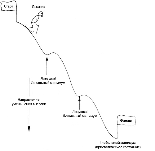
Let us imagine for a moment a skier, rushing along the steep slope of our objective function. The task is to go down to the lowest point (global minimum). But, as you can see, the slope we got was not quite even, there are lowlands on it, having come to them, it may seem to us that we are already at the foot. In order not to stay in the cold, we will have to show curiosity and climb a small mound to continue the descent.
In order for the metaphor to be finally understood, in the skier example, the slope is the function of measuring the energy of a substance (it is the objective function). A probabilistic transition to a state with more energy - climbing on a hill to the right of the lowlands.
As you can see, such an algorithm allows us with a high probability to avoid “getting stuck” in the local minimum.
Now we are ready to move to a more rigorous description of the method. We introduce the notation:
Let S be the set of all states (solutions) of our problem. For example, for the knapsack problem, this will be a multitude of various sets of things.
Let be - state on the i-th step of the algorithm.
  .
.
 - temperature at the i-th step.
In order to use the annealing simulation, we need to define three functions:
Now we will dwell on each detail.
E to each decision according to some rule puts a number in correspondence. Depends on the specific task.
T sets the iteration number i to the corresponding temperature. The function determines how long our algorithm will work (in fact, it has a deeper meaning, but for now we don’t need to know this). If T is a linear function, then the running time will be relatively large. In the case of a power function, say , everything will end very quickly, but it is far from a fact that we will not get stuck in the lowlands, so not having reached the finish line.
For this article, I chose the simplest, linear option.
At once I will make a reservation that all the code in this article was written on Matlab . I chose this medium, as out of the box you can draw beautiful graphics - no more. I tried to write without using specific matlab magic so that the code could be easily ported to your favorite language.
The function F, based on the previous state, generates a new candidate state, into which the system can go, and it can also drop it. Denote it . The method of obtaining a candidate depends entirely on the problem being solved, you can see a specific function in the example.
Now we can describe the algorithm of the simulated annealing method in the most general form:
As you can see, everything is very simple, it is worthwhile to separately explain only the transition to a new state. If the energy of the “candidate” is less, it becomes a new state, otherwise, the transition will be probabilistic (therefore, the method is referred to the stochastic class).
So that this does not cause any difficulties, I will allow myself to recall some of the most basic concepts of probability theory.
We informally define the probability as a measure of the possibility of the occurrence of a certain event. The probability of a reliable event (an event that just happens) is equal to one, the impossible - zero. All other values are between.
For example, when throwing a die, the probability of dropping any number is one, and triples - 1/6.
In our case, substituting the energy difference values in the formula and temperatures
  we get the probability of transition. It remains only to make this transition, but how to do it?
Probability calculation code:
Let's imagine a single segment and divide it into two parts relative to the value of our probability.

Then we use the function of generating a uniformly distributed random number, in Matlab this is rand (as in almost all other languages). Now we note this number on the segment.

If the number is in the left part - we make the transition, in the right - we do not do anything.
Now, I think everything is clear, and we can go directly to the solution of our first task.
Imagine that you are a wandering merchant and want to offer your goods to the inhabitants of every city in the country. Traveling takes a lot of time and effort, so it is logical that you want to make your route in such a way that the distance to be covered is minimal. This route is to be found.
More formally: you need to find the shortest path that passes through each city and ends at the point of departure.
In this formulation, the problem is called the closed-door traveling salesman problem.
First, let's define the data. Let our cities be randomly scattered in a 10x10 square. Each city, respectively, is represented by a pair of coordinates. Only 100 cities.

Data can be easily obtained in Matlab with the following code:
In other languages, you have to write a cycle, but in fact it does not change anything. We generate random numbers with the rand () function already familiar to us and multiply them by 10 so that they lie in a given area.
Denote the set of all cities by C, the total number is denoted by | C | and in our case it is 100. Every city represented as a pair of coordinates
  with the appropriate index.
By convention, the solution is a route between all cities, which means the set of states S are all possible routes passing through each city. In other words, the set of all ordered sequences of elements of C, in which any occurs exactly once. Obviously, the length of each such sequence | C |.
As we remember, in order to use the method of simulating annealing, we must define two functions depending on each specific task. This is the energy function E (or the “objective function” in the common terminology) and the function F generating the new state.
As we strive to minimize the distance, it will be “energy”. Therefore, our objective function will be as follows:

It says nothing more than the sum of the Euclidean distances between pairs of cities in the route . Since the task is closed, we were forced to sign
  at the end, this is the distance between the last and the first city. If you do not go deep, then Euclidean is the very distance between points that we all went through in geometry lessons. It is given by the following formula:

Where
Now let's think about how we get a new state? The first thing that comes to mind is to swap two arbitrary cities in the route. The idea is correct, but such a change unpredictably affects , the method will work for a long time and not the fact that it is successful.
A good option in this case would be to choose two arbitrary cities in the route and invert the path between them. For example, we had a route (1,2,3,4,5,6,7). The random number generator chose cities 2 and 7, we performed the procedure and got (1,7,6,5,4,3,2).
Below is the code for function F:
Now we have everything we need, and we can start the optimization process. But before we go to the most interesting, I will give the full program code. I think it would be very interesting to compare it with the above pseudocode paragraph pair:
As you can see, nothing complicated.
Since the algorithm has a probabilistic nature, the case can be ordered so that the “annealing” will take, and even get stuck in a local minimum. Therefore, it is worth making several launches and paying attention to what minimum value the results converge.
The program started with = 10 and
  = 0.00001.
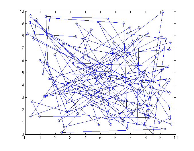
The figure shows the state at the very first iteration. It is unlikely that the salesman would have experienced great joy, we offer him such a route.
The output result looks much nicer:
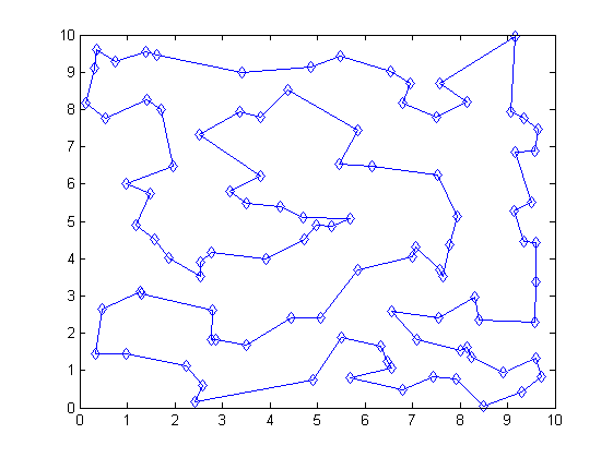
However, it is worth noting that in spite of the fact that the algorithm in the current implementation works quite efficiently (exactly much faster than exhaustive search), it is believed that much better time can be achieved without losing “quality”. To do this, I suggest you, as a practical task, experiment with the T function and share the results in the comments.
Source codes can be downloaded here .
I hope that the read turned out to be useful for you. Constructive criticism is welcome.
PS
Taking this opportunity, I would like to thank Anna Antonova and Dmitry Ignatov, who read the article before publication and gave me some good advice.
To understand the article, you will need minimal programming skills and mastery of mathematics at the grade 9 level of high school. The article is intended for people who are not familiar with optimization methods or who are just taking the first steps in this direction.

')
In order to maximize the circle of readers, I had to almost completely abandon formal definitions and consciously go for some not entirely accurate simplifications. I hope that with the water I did not throw out the child (and if this happened, I will be glad to your comments).
About optimization
In order to understand what optimization is, you first need to know what it is for. At once I will say that with the “optimization problems” in everyday life we are confronted with enviable regularity, without giving ourselves a report on this.
Suppose we, having received the next salary, decide to line up the family budget. It is necessary to allocate money so that first of all to satisfy the most important needs (food, electricity, Internet, etc.), and the rest can be lowered to something lower priority. Buy all the money designer phone and die of hunger - not the best solution, is not it?
Or another option, we decided to go hiking and collect a satchel. One problem is that there is a lot of things, and our backpack is not too big (and we ourselves have limited carrying capacity). We want to take as many of the most important items for us as possible. If we go to the mountains, grabbing a safety cable with us is a good decision, take your favorite PlayStation Vita instead, and probably don’t give you the rest of the time with cookies.
So what does the optimization do? She is looking for the very good solution. Perhaps not the best of all, but definitely good.
Now a little bit more formal. If you look at Wikipedia, you can easily find the following definition:
The optimal (from the Latin. Optimus - the best) solution - a solution that, in one way or another, is preferable to others. Therefore, optimization is a way to find the optimal solution.
Now, let's imagine that we can measure how good our decision is. For example, in the case of a “knapsack problem”, we assign each thing a natural number (the larger the number, the more important the thing). Then our task gets a clearer statement: we want to fill the satchel with such things, the total priority of which will be maximum, and the weight will not exceed a certain value. Those. we are looking for the maximum of a certain function , which is called the target .
To reduce everything to a common denominator, look again at Wikipedia:
Optimization (mathematics) - finding the extremum (minimum or maximum) of the objective function in a certain area.
Now that we have more or less decided on what the optimization is doing, a reasonable question appears - “How?”.
Of course, we can not particularly bother and go through all the solutions, and then compare them. In the case of the knapsack, we can probably even do this. But now let's imagine that our satchel is not a satchel at all, but a whole train with many wagons, but we transport different goods to another city. The task has not changed (load as much as possible valuable), and the target function will be the total value of the goods. How long will it take us to complete a bust of solutions? I think a lot.
You can choose solutions randomly. Suppose there are a hundred solutions, and then take the best of them. Undoubtedly, it will be much faster than complete enumeration, but who will guarantee that our final solution will be at all close to the extremum?
I will not torment and say that there are a great many optimization methods . So much that they are usually divided into classes, I will not list them all. Let me just say that “annealing imitation” refers to the class of stochastic (from the Greek. Στχχσστικός - “ able to guess ”) or probabilistic methods. And where is the probability and how it will help find a solution - just below.
Annealing imitation
Like all brilliant, this method is peeped at Mother Nature. It is based on the process of crystallization of the substance, which in turn was “tamed” by sly metallurgists, in order to increase the homogeneity of the metal.
Let me remind you that every metal has a crystal lattice , if very briefly, it describes the geometric position of the atoms of matter. The set of positions of all atoms will be called the state of the system, each state corresponds to a certain level of energy. The purpose of annealing is to bring the system to the lowest energy state. The lower the energy level, the “better” the crystal lattice, i.e. the fewer defects and stronger the metal.
During the "annealing" the metal is first heated to a certain temperature, which causes the atoms of the crystal lattice to leave their positions. Then begins a slow and controlled cooling. Atoms tend to get into a state with less energy, however, with a certain probability they can go into a state with more. This probability decreases with temperature. The transition to the worst state, oddly enough, helps in the end to find a state with energy less than the initial one. The process ends when the temperature drops to a predetermined value.
As you can see, in the framework of this process, energy is minimized. We change the energy to our target function, and voilà! Or not? Let's think, and why is so tricky process so good? Why don't we, for example, always go to lower energy states?
This is how the gradient descent method works widely.
On the Internet, I managed to find a completely wonderful picture that illustrates the best of the algorithm.

Let us imagine for a moment a skier, rushing along the steep slope of our objective function. The task is to go down to the lowest point (global minimum). But, as you can see, the slope we got was not quite even, there are lowlands on it, having come to them, it may seem to us that we are already at the foot. In order not to stay in the cold, we will have to show curiosity and climb a small mound to continue the descent.
In order for the metaphor to be finally understood, in the skier example, the slope is the function of measuring the energy of a substance (it is the objective function). A probabilistic transition to a state with more energy - climbing on a hill to the right of the lowlands.
As you can see, such an algorithm allows us with a high probability to avoid “getting stuck” in the local minimum.
Now we are ready to move to a more rigorous description of the method. We introduce the notation:
Let S be the set of all states (solutions) of our problem. For example, for the knapsack problem, this will be a multitude of various sets of things.
Let be
 - state on the i-th step of the algorithm.
  .
. - temperature at the i-th step.
In order to use the annealing simulation, we need to define three functions:
- The function of energy or, more simply, what we optimize.

- The function of temperature changes over time. Just in case, make a reservation that it must be decreasing.

- The function that generates the new state.

Now we will dwell on each detail.
E to each decision according to some rule puts a number in correspondence. Depends on the specific task.
T sets the iteration number i to the corresponding temperature. The function determines how long our algorithm will work (in fact, it has a deeper meaning, but for now we don’t need to know this). If T is a linear function, then the running time will be relatively large. In the case of a power function, say
 , everything will end very quickly, but it is far from a fact that we will not get stuck in the lowlands, so not having reached the finish line.
For this article, I chose the simplest, linear option.
function [ T ] = DecreaseTemperature( initialTemperature, i) %initialTemperature - %i - T = initialTemperature * 0.1 / i; end At once I will make a reservation that all the code in this article was written on Matlab . I chose this medium, as out of the box you can draw beautiful graphics - no more. I tried to write without using specific matlab magic so that the code could be easily ported to your favorite language.
The function F, based on the previous state, generates a new candidate state, into which the system can go, and it can also drop it. Denote it
 . The method of obtaining a candidate depends entirely on the problem being solved, you can see a specific function in the example.
Now we can describe the algorithm of the simulated annealing method in the most general form:
- Inlet: minimum temperature
 initial temperature
- Set an arbitrary first state


- Until


- If a
 then
then 
- If a
 the transition is carried out with probability
- Lower the temperature

- Return the last state s
As you can see, everything is very simple, it is worthwhile to separately explain only the transition to a new state. If the energy of the “candidate” is less, it becomes a new state, otherwise, the transition will be probabilistic (therefore, the method is referred to the stochastic class).
So that this does not cause any difficulties, I will allow myself to recall some of the most basic concepts of probability theory.
We informally define the probability as a measure of the possibility of the occurrence of a certain event. The probability of a reliable event (an event that just happens) is equal to one, the impossible - zero. All other values are between.
For example, when throwing a die, the probability of dropping any number is one, and triples - 1/6.
In our case, substituting the energy difference values in the formula
 and temperatures
  we get the probability of transition. It remains only to make this transition, but how to do it?
Probability calculation code:
function [ P ] = GetTransitionProbability( dE, T ) P = exp(-dE/T); end Let's imagine a single segment and divide it into two parts relative to the value of our probability.

Then we use the function of generating a uniformly distributed random number, in Matlab this is rand (as in almost all other languages). Now we note this number on the segment.

If the number is in the left part - we make the transition, in the right - we do not do anything.
function [ a ] = IsTransition(probability) value = rand(1); if(value <= probability) a = 1; else a = 0; end end Now, I think everything is clear, and we can go directly to the solution of our first task.
Traveling salesman task
Imagine that you are a wandering merchant and want to offer your goods to the inhabitants of every city in the country. Traveling takes a lot of time and effort, so it is logical that you want to make your route in such a way that the distance to be covered is minimal. This route is to be found.
More formally: you need to find the shortest path that passes through each city and ends at the point of departure.
In this formulation, the problem is called the closed-door traveling salesman problem.
First, let's define the data. Let our cities be randomly scattered in a 10x10 square. Each city, respectively, is represented by a pair of coordinates. Only 100 cities.

Data can be easily obtained in Matlab with the following code:
data = rand(2,100)*10; In other languages, you have to write a cycle, but in fact it does not change anything. We generate random numbers with the rand () function already familiar to us and multiply them by 10 so that they lie in a given area.
Solving the problem by simulating annealing
Denote the set of all cities by C, the total number is denoted by | C | and in our case it is 100. Every city
 with the appropriate index.
By convention, the solution is a route between all cities, which means the set of states S are all possible routes passing through each city. In other words, the set of all ordered sequences of elements of C, in which any
As we remember, in order to use the method of simulating annealing, we must define two functions depending on each specific task. This is the energy function E (or the “objective function” in the common terminology) and the function F generating the new state.
As we strive to minimize the distance, it will be “energy”. Therefore, our objective function will be as follows:

It says nothing more than the sum of the Euclidean distances between pairs of cities in the route
 . Since the task is closed, we were forced to sign
  at the end, this is the distance between the last and the first city. If you do not go deep, then Euclidean is the very distance between points that we all went through in geometry lessons. It is given by the following formula:
Where

Now let's think about how we get a new state? The first thing that comes to mind is to swap two arbitrary cities in the route. The idea is correct, but such a change unpredictably affects
 , the method will work for a long time and not the fact that it is successful.
A good option in this case would be to choose two arbitrary cities in the route and invert the path between them. For example, we had a route (1,2,3,4,5,6,7). The random number generator chose cities 2 and 7, we performed the procedure and got (1,7,6,5,4,3,2).
Below is the code for function F:
function [ seq ] = GenerateStateCandidate(seq) %seq - (), % - n = size(seq,1); % i = randi(n,1); % j = randi(n, 1);% if(i > j) seq(j:i) = flipud(seq(j:i)); % else seq(i:j) = flipud(seq(i:j));% end end Now we have everything we need, and we can start the optimization process. But before we go to the most interesting, I will give the full program code. I think it would be very interesting to compare it with the above pseudocode paragraph pair:
function [ state ] = SimulatedAnnealing( cities, initialTemperature, endTemperature) n = size(cities,1); % state = randperm(n); % , % randperm(n) - 1 n currentEnergy = CalculateEnergy(state, cities); % T = initialTemperature; for i = 1:100000 % % T stateCandidate = GenerateStateCandidate(state); % - candidateEnergy = CalculateEnergy(stateCandidate, cities); % if(candidateEnergy < currentEnergy) % currentEnergy = candidateEnergy; % state = stateCandidate; else p = GetTransitionProbability(candidateEnergy-currentEnergy, T); % , if (MakeTransit(p)) % , currentEnergy = candidateEnergy; state = stateCandidate; end end; T = DecreaseTemperature(initialTemperature, i) ; % if(T <= endTemperature) % break; end; end end As you can see, nothing complicated.
results
Since the algorithm has a probabilistic nature, the case can be ordered so that the “annealing” will take, and even get stuck in a local minimum. Therefore, it is worth making several launches and paying attention to what minimum value the results converge.
The program started with
 = 10 and
  = 0.00001.
The figure shows the state at the very first iteration. It is unlikely that the salesman would have experienced great joy, we offer him such a route.

The output result looks much nicer:

However, it is worth noting that in spite of the fact that the algorithm in the current implementation works quite efficiently (exactly much faster than exhaustive search), it is believed that much better time can be achieved without losing “quality”. To do this, I suggest you, as a practical task, experiment with the T function and share the results in the comments.
Source codes can be downloaded here .
I hope that the read turned out to be useful for you. Constructive criticism is welcome.
PS
Taking this opportunity, I would like to thank Anna Antonova and Dmitry Ignatov, who read the article before publication and gave me some good advice.
Source: https://habr.com/ru/post/209610/
All Articles