Physical design of storage structures in Teradata DBMS

What is the physical design of storage structures?

The main goal pursued during the development of a physical data model is the creation of such objects for a specific platform / DBMS, which will achieve maximum performance of queries / applications that create the main load, while reducing additional costs, such as the need to maintain additional indices, to materialize derivatives. data, etc., to a minimum.
All relational databases are built on the same principles, but each platform has unique features in the form of the presence of various types of objects and features of their implementation. For this reason, the process of physical modeling is platform-specific, in contrast to logical modeling, the main purpose of which is to reliably describe data and business processes.

Data Storage in Teradata DBMS

Speaking about the physical design of databases on the Teradata platform, among other things, it is necessary to mention that this is a MPP (Massive Parallel Processing) platform in which all data is distributed among the system components (AMPs) and processed by them when executing user queries in parallel (see our first article ). This architecture, as well as the even distribution of the data, make their processing efficient and in the absence of additional performance elements. This feature allows Teradata to cope perfectly with Ad-Hoc requests not provided for by the developers of the physical model.
But for mixed loads, when both tactical (OLTP-like) and strategic (OLAP, DSS, Data Mining) requests are executed simultaneously on the system, this is not enough. This especially applies to tactical requests that have sufficiently high requirements for response time and throughput. The main technique of physical design to improve the performance of tactical queries is the creation of indexes — data access paths that can be used by queries to quickly find the right rows of a table without having to look at it completely. The use of indexes allows you to drastically reduce the number of I / O operations during query execution, which reduces response time and, as a result, increases system throughput. Let's take a look at how the indexes are arranged in Teradata, taking into account the parallel architecture.

Ways to access data

DBMS Teradata supports various ways to access rows of tables:
')

Access by the primary index (what the primary index is, was discussed in our first article )

This is the fastest and least expensive way to access data in Teradata.
Recall that the data in the Teradata DBMS is distributed using the result of hashing the value of the column of the primary index. Rows with the same values ​​of the column of the primary index ALWAYS fall on the same AMP.

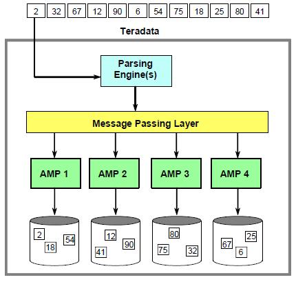
The algorithm used to determine AMP, on which a row should be placed when it is inserted into a table, is equally well used to search for a row with a known value of the column of the primary index.

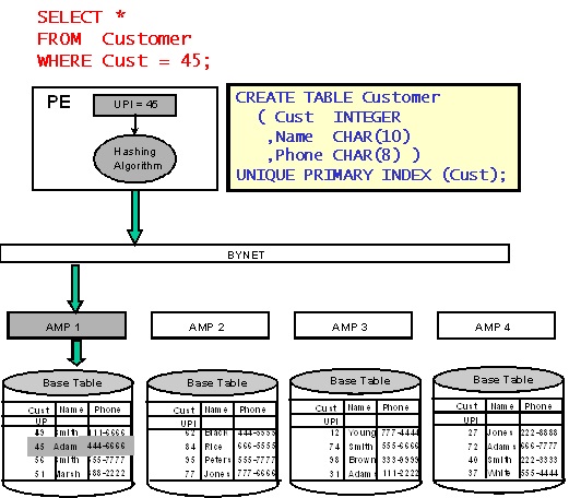
When the AMP on which the search string is located is defined, Teradata uses index structures to find the required data block. Sequentially viewed:

• Master Index (always loaded into AMP memory) to search for a cylinder containing the required data block;
• Cylinder Index (almost always loaded into AMP memory) to search for the desired data block.

After the required data block is found, it is read and then the string is searched using an array of row pointers (Row Reference Array).

This algorithm works equally for both unique (Unique Primary Index - UPI) and non-unique (Non-unique Primary Index - NUPI) primary indexes - with the only difference that when accessing via UPI, only one data block is always read and no more single line, while accessing by NUPI these values ​​depend on the degree of nonuniqueness of the index.

Base table row format


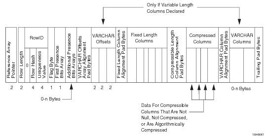
The peculiarity of data storage in Teradata is that on each AMP, the rows of the tables are not stored in an arbitrary order, but are sorted by the hash values ​​of the primary index. Such an approach requires additional efforts when inserting data, since new rows should be inserted not into the “end of the table”, but so as to preserve sorting by hashes. In this case, we get two advantages:

• When joining the primary index column, you can immediately apply the effective MERGE JOIN join, since the rows are already ordered.
• Automatic indexing of the primary index column. The internal file system indexes (master index and cylinder index), mentioned above, contain within the range of hash values ​​for the data stored in data blocks. Due to the fact that the rows are ordered, these ranges do not overlap. As a result, by creating disk space markup for data blocks, we actually get not only this markup itself, but also the indexing of the primary index column — the classic B-tree index by the hash values ​​of the primary index. We sometimes even say that the primary index does not occupy disk space and does not require maintenance, bearing in mind that it is part of the master index and cylinder index structure for storing data on the AMP disk system.

The features of this algorithm also determine the limitations inherent in it, namely, access by the primary index is possible only under the following conditions:

• using the condition "equal" in the query to filter on the column of the primary index;
• inclusion in the search conditions of ALL columns constituting the primary index.

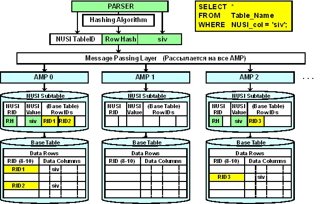
Access by secondary index

Secondary indexes are alternative data access paths. Implemented in the form of index sub-tables, which allow identifying the corresponding identifiers of rows of the base table by the value of the indexing column.

The implementation of the index sub-tables of the unique (Unique Secondary Index - USI) and non-unique (Non-unique Secondary Index - NUSI) secondary indexes differ.

USI index sub-table row format


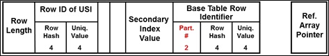
The rows of the USI index sub-table are distributed across the AMPs using the index hashing result. With high probability, the row of the index table will be on a different one with respect to the corresponding row of the base table AMP. Each row in the base table corresponds to a row in the index sub-table. Access to data using USI requires the involvement of two AMPs (the first to search for the row in the index, the second to read the row of the base table by its identifier). Data access using USI can be considered as effective as using a primary index. The main purpose of USI is data access by index column value. In the same way, as for the primary index, in the expression "WHERE" ALL columns should be specified that make up the index with the condition "EQUAL".



NUSI index sub-table row format



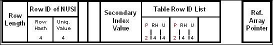
The rows of the index sub-table NUSI are located locally (on the same AMPs) with respect to the rows of the base table and are logically sorted by default by the hash value of the secondary index column. Such storage means that the rows with the same value of the index column can be found on any of the AMPs of the system, and, therefore, all AMPs will be involved in the search for the required rows in the index subtable. Further, to select rows from the base table, only those AMPs will be used, on which the rows of the index sub-table are selected. Whether the optimizer will use NUSI for data access depends on the selectivity of the index. As a value, above which the optimizer chooses a full table scan, you can rely on 1% (if, when executing the query, less than 1% of the table rows are selected, the index will be used). The rule from this follows: collect statistics on NUSI, without them the optimizer will select FTS.



As in the case of PI and USI, by default NUSI is used to access rows by value (the “EQUAL” condition on all NUSI columns in the “WHERE” expression). But besides this, NUSI can also be used for queries with range access to rows of a table, for which there is an option “ORDER BY VALUES”, which logically sorts the rows of the index sub-table by the value of the index column. The index created in such a way allows to increase the performance with the conditions on the index column different from "EQUAL": <,>,> =, <=, BETWEEN.

Also, as you can see from the format of the row of the index sub-table, there can be more than one RowID of the base table per index column value. This makes the index sub-table NUSI automatically compressible, which minimizes the used disk space.

Full table scan (Full Table Scan, or FTS)
There is nothing to say about this access method. Teradata uses it in cases where other data access paths, from the point of view of the optimizer, are inefficient. I just want to note that the search for strings through a full scan in Teradata is very effective thanks to the MPP architecture, since many AMPs simultaneously scan distributed table fragments. Often, a complete reading of tables containing millions of rows requires each AMP to perform only a few I / O operations.

Concluding this review of access to the data of the primary / secondary index tables, we would like to note that Teradata, in the presence of alternatives, will always prefer the primary index to the secondary and unique to the non-unique one.



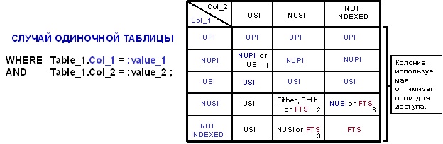
1. The optimizer prefers the primary index to the secondary index, and the unique indexes - non-unique. NUPI will be given preference only if one data block (1 I / O) is requested.
2. Depending on the selectivity, the optimizer may use NUSI, NUSI Bit Mapping or FTS.
3. It all depends on the selectivity of the index.

Access with join of tables

Another way to access data is to join two or more tables. This process has one very important feature specific to MPP platforms. It lies in the fact that the connection tables are AMP'ami, and the data involved in the connection must be on the corresponding AMP'ah.
As you remember, the distribution of rows of the table by AMPs depends on the primary index, and the rows of the joined tables with the same values ​​of the connection column are not always located on the same AMPs. Therefore, it is not always, but often, a table join is preceded by a preparatory operation. An exception is the combination of two tables on the primary index column, since in this case the rows with the same values ​​of the primary index columns are already on the same AMP. Joining tables by PI column is the fastest.

In all other cases, to perform a table join, Teradata can ensure that there are rows on the same AMP with the same value of the join column in the following ways (important: all derived data sets are materialized in SPOOL - the temporary storage area for intermediate query results):

• duplication of rows of a small table for all amps;
• reallocation of rows of one / both tables of a join step by a connection column (change of PI). In this case, the table itself remains in place, and a temporary copy of the rows that participate in the query (not necessarily the entire table) is created, with a different primary index.
  Which of the above methods will be chosen by the optimizer depends on the data demographics, the availability of collected statistics and indexes (Teradata may use certain types of indices, for example, NUSI, to improve the performance of the compounds).

When the availability of the necessary data on the AMPs is assured, Teradata can use traditional table join strategies such as:

• MERGE JOIN:
  • Row Hash;
  • Inclusion;
  • Exclusion;
• PRODUCT JOIN;
• NESTED JOIN;
• HASH JOIN.

What you need to have to perform high-quality physical design

Logical model

Directly physical modeling is traditionally preceded by the creation of a logical model, which later serves as a template for creating database objects. The structure of a good logical model can be implemented in a one-to-one database.
For corporate data warehouses, the logical model is a description of all the business processes of an organization. It should be implemented in such a way as to not only solve existing business problems, but also support its further development. Creating such a model from scratch is a very nontrivial and time-consuming task, requiring excellent knowledge of the subject area and modeling techniques. In this article, we will not discuss issues of logical modeling; we only note that in our projects we try to use the industry-specific Teradata logical models tested by time and numerous implementations. To those who consider Western models unsuitable for use on the Russian market, we can say that in practice the scope of localization (or, better to say, the adaptation of the model to customer processes, since organizations with identical processes are rarely found) is small and often reduces to the expansion of the attribute structure entities already in the model.

Data

No, you can, of course, model “in vacuum”, but for the physical model it is extremely important to have data before your eyes that will later be loaded into the model. This allows you to make decisions about how to move from a logical model to a physical one. Some believe that the one-to-one physical model corresponds to the logical one, but this is far from always the case. For example, as a result of data analysis, it may be decided to implement several entities of the logical data model in the form of a single table in a physical table. And this is just one example.

Demographics

No matter how good the logical model may be, it is not enough just a set of entities and relationships to perform a high-quality physical design — an understanding of the specifics of the data and the nature of their use is necessary. Usually we analyze several demographics:

• data demographics — data volumes, frequency diagrams, etc .;
• demography of variability - how often data changes in a particular column of the table;
• Usage demographics — whether columns are used to access data by value (single or range of values) or by connection.

Knowledge of the above demographics allows the creator of a physical model to make a choice consciously.
Obviously, not all of these demographics are known before using the model. In particular, the methods of accessing data and the frequency of accessing one or another column of the model at 100% 99% can only be learned after a long period of storage operation. But a fairly large number of access methods can be thought out in advance, based on the implementation logic of the model itself.

Patience and attentiveness

Physical modeling is a fascinating process, but not always clearly algorithmic. Paraphrasing the character of a famous Soviet cartoon: "Physical modeling is not an exact science." On the one hand, this provides opportunities for creativity, on the other hand, it takes time, care and, often, an iterative approach, so attention to detail and patience when working with large data models play a key role in physical modeling.

Index selection

Indices are often used as one of the main ways to optimize the physical model for certain patterns of use. Sometimes the choice of indexes may seem obvious. Let's look at an example where the obvious is not always true.
Imagine the following table: ACCOUNT (1,000,000 lines)

Acct_id	Acct_num	Acct_open_dt	Acct_close_dt	Acct_pty_id
PK	NOT NULL, UNIQUE	NOT NULL		NOT NULL, FK
UPI	USI	Nusi	NUSI?	Nusi

The third line contains the intended choice of indexes.
Legend:

• UPI (Unique Primary Index)
• NUPI (Non-Unique Primary Index)
• USI (Unique Secondary Index)
• NUSI (Non-Unique Secondary Index)

Can you say with certainty that this choice is the right one? I think that the experience of creating physical models for a particular DBMS can suggest the right choice, but in the general case it cannot be said that the choice made is correct. Speaking about the example presented above, you can, for example, ask yourself whether a search is performed in this table by account identifier? If the answer is no, you can exclude the Acct_id column from the candidates for the primary index.
A simple example shows that even the best logical model is not enough to create a physical model. An understanding of the data demographics is required (see above). Let's add the demographics to the example above and see if this makes it easier.
Same ACCOUNT table (1,000,000 rows)

	Acct_id	Acct_num	Acct_open_dt	Acct_close_dt	Acct_pty_id
	PK	NOT NULL, UNIQUE	NOT NULL		NOT NULL, FK
Frequency of access by value	800	10K	1K	500	1K
Connection Frequency	3K	0	0	0	5K
Number of unique lines	1000K	1000K	731	256	400K
Max. number of lines per value (non-NULL)	one	one	2056	1K	7
Typical number of lines per value	one	one	1235	400	2
Number of lines with NULL	0	0	0	900K	0
Intended choice	UPI	USI	Nusi	Nusi	Nusi
Select based on demographics	Nusi	USI	Nusi	NUSI?	NUPI

As you can see, the initial selection of indexes has been changed. There are quite objective reasons for this:

• For Acct_pty_id column
  Access by primary index is the most effective method of accessing data in Teradata. As we see from the example, access by the value of this column occurs frequently. In addition, the same column is most often used to connect to another table. Joining two tables along primary index columns is also most preferable for Teradata.
• For Acct_id column
  This column is also used for access quite often. Since the choice of the primary index has already been made, we can create a non-unique secondary index for the most efficient reading of the rows of the table by value and improving the performance of the connections.
• For Acct_close_dt column
  The choice of the index is questioned due to the fact that at certain values ​​(NULL) Teradata will not use it due to insufficient selectivity.

Partitioning tables in Teradata

If the table is large in size, then the natural desire is to break it into parts (partitions) and scan only these partitions instead of a full view of the table.
In Teradata, the following two mechanisms — distribution across AMPs and partitioning — effectively complement each other. Partitioned tables are distributed by AMPs in the same way as nonpartitioned tables. Further, on each AMP, the lines are ordered first by partitions, and the part numbers are written into the master index and cylinder index for addressing data blocks. And then, within the partitions, the rows are already sorted by the hash values ​​of the primary index, as well as for nonpartitioned tables.
Thus, if we launch a query of the form “BETWEEN value_1 AND value2” of the column_partitioning, then all AMPs work in parallel and scan each fragment of the table, but not completely, but only the necessary partitions.
There is also a multi-level partitioning, when there are several columns, and subpartitions are created inside the partitions.
All large tables are usually partitioned. This physical design technique can improve the performance of certain queries that have filtering by partitioning fields.

Conclusion

In this article, we decided to limit ourselves to the description of the basic principles and elements used in the implementation of the physical database design for the Teradata DBMS. Using only these practices in the work will allow those who are just starting to work with massively parallel DBMSs not to step on the “rake” at the very beginning of the journey.
In the next article, “Additional Physical Modeling Techniques in Teradata,” we plan to tell you about additional features for indexing and compressing data in Teradata.
We are waiting for your questions.