Converting a uniformly distributed random variable to a normally distributed one
This question has long been studied in detail, and the polar coordinate method proposed by George Box, Mervin Muller and George Marsaly in 1958 was most widely used. This method allows to obtain a pair of independent normally distributed random variables with a mean of 0 and variance 1 as follows:
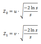
where Z 0 and Z 1 are the desired values, s = u 2 + v 2 , and u and v are random variables uniformly distributed on the segment (-1, 1), chosen in such a way that the condition 0 <s <1 is met.
Many use these formulas without even thinking, and many do not even know about their existence, since they use ready-made implementations. But there are people who have questions: “Where did this formula come from? And why do you get a couple of values right away? ” Next, I will try to give a clear answer to these questions.
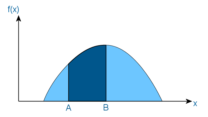
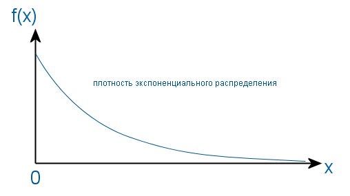
To begin, let me remind you what probability density, the distribution function of a random variable, and the inverse function are. Suppose there is some random variable whose distribution is given by the density function f (x), which has the following form:
')
This means that the probability that the value of this random variable will be in the interval (A, B) is equal to the area of the shaded area. And as a result, the area of the entire shaded area should be equal to one, since in any case the value of a random variable falls within the domain of definition of the function f.
The distribution function of a random variable is an integral of the density function. And in this case, its approximate form would be:
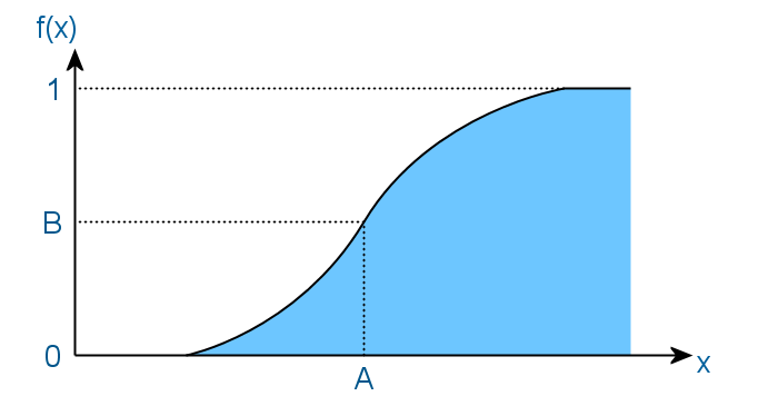
Here the meaning is that the value of a random variable will be less than A with probability B. And as a result, the function never decreases, and its values lie in the interval [0, 1].
The inverse function is a function that returns the argument of the source function, if the value of the source function is passed to it. For example, for the function x 2, the inverse will be the root extraction function, for sin (x) this is arcsin (x), etc.
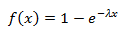
Since most of the generators of pseudo-random numbers at the output give only a uniform distribution, it is often necessary to convert it to some other one. In this case, in a normal Gaussian:
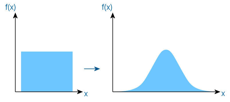
The basis of all methods of converting a uniform distribution to any other is the method of inverse transformation. It works as follows. A function is found which is the inverse of the required distribution function, and a random variable uniformly distributed on the segment (0, 1) is passed to it as an argument. At the output, we obtain a value with the required distribution. For clarity, bring the following picture.

Thus, a uniform segment is smeared in accordance with the new distribution, projecting onto another axis through the inverse function. But the problem is that the integral of the density of the Gaussian distribution is not easy to calculate, so the above scientists had to cheat.
There is a chi-square distribution (Pearson distribution), which is the distribution of the sum of squares of k independent normal random variables. And in the case when k = 2, this distribution is exponential.
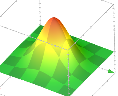
This means that if a point in the rectangular coordinate system has random coordinates X and Y distributed normally, then after transferring these coordinates to the polar system (r, θ) the square of the radius (distance from the origin of coordinates to the point) will be distributed exponentially since the square of the radius is the sum of the squares of the coordinates (according to the law of Pythagoras). The density of distribution of such points on the plane will look as follows:
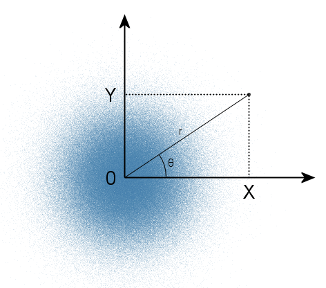
Since it is equivalent in all directions, the angle θ will have a uniform distribution in the range from 0 to 2π. The reverse is also true: if you specify a point in the polar coordinate system using two independent random variables (an angle distributed uniformly and a radius distributed exponentially), then the rectangular coordinates of this point will be independent normal random variables. And the exponential distribution from the uniform is already much easier to obtain using the same inverse transform method. This is the essence of the polar Box-Muller method.
Now we derive the formulas.
 (one)
(one)
To obtain r and θ, we need to generate two randomly distributed random variables on the segment (0, 1) (we will call them u and v), the distribution of which one (say v) should be converted to exponential to obtain the radius. The exponential distribution function is as follows:
Back to her function:
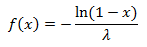
Since the uniform distribution is symmetrical, then the transformation will work in the same way as
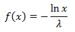
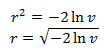
From the chi-square distribution formula, it follows that λ = 0.5. Substitute λ, v into this function and get the square of the radius, and then the radius itself:
The angle we get, stretching a single segment to 2π:

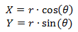
Now we substitute r and θ into formulas (1) and we get:
 (2)
(2)
These formulas are ready to use. X and Y will be independent and normally distributed with variance 1 and expected value 0. To get a distribution with other characteristics, it is enough to multiply the result of the function by the standard deviation and add the expected value.
But it is possible to get rid of trigonometric functions by setting the angle not directly, but indirectly through the rectangular coordinates of a random point in a circle. Then through these coordinates it will be possible to calculate the length of the radius vector, and then find the cosine and sine, dividing x and y into it, respectively. How and why does it work?
Choose a random point from uniformly distributed in a circle of unit radius and denote the square of the length of the radius vector of this point by the letter s:
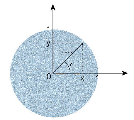
The choice is made by specifying random rectangular coordinates x and y, uniformly distributed in the interval (-1, 1), and discarding points that do not belong to a circle, as well as a central point at which the angle of the radius vector is not defined. That is, the condition 0 <s <1 should be satisfied. Then, as in the case of the Gaussian distribution on the plane, the angle θ will be uniformly distributed. This is obvious - the number of points in each direction is the same, so each corner is equally likely. But there is a less obvious fact - s will also have a uniform distribution. The resulting s and θ will be independent of each other. Therefore, we can use the value of s to obtain an exponential distribution without generating a third random variable. We now substitute s into formulas (2) instead of v, and instead of trigonometric functions, their calculation by dividing the coordinate by the length of the radius vector, which in this case is a root of s:

We get the formulas, as in the beginning of the article. The disadvantage of this method is to drop points that are not included in the circle. That is, using only 78.5% of the generated random variables. On older computers, the lack of trigonometric functions still gave a big advantage. Now, when one team of a processor calculates both sine and cosine in an instant, I think these methods can still compete.
Personally, I still have two questions:
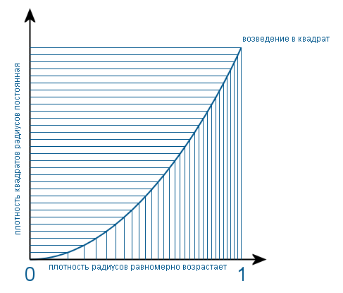
Since s is the square of the radius (for simplicity, I call the length of the radius vector specifying the position of a random point the radius), we first find out how the radii are distributed. Since the circle is filled uniformly, it is obvious that the number of points with a radius r is proportional to the length of a circle of radius r. And the circumference is proportional to the radius. So the density distribution of the radii increases uniformly from the center of the circle to its edges. And the density function has the form f (x) = 2x on the interval (0, 1). Coefficient 2 so that the area of the figure under the graph is equal to one. When such a density is squared, it becomes uniform. Since theoretically, in this case, it is necessary to divide the density function by the derivative of the transformation function (that is, x 2 ). And clearly it happens like this:
If we make a similar transformation for a normal random variable, then the density function of its square will be similar to a hyperbola. And the addition of two squares of normal random variables is a much more complicated process associated with double integration. And the fact that the result will be an exponential distribution, I personally need to check here with a practical method or accept it as an axiom. And to whom it is interesting, I suggest that you familiarize yourself with the topic, drawing on the knowledge from these books:
In conclusion, I will give an example of the implementation of a generator of normally distributed random numbers in the JavaScript language:
The parameters mean (mathematical expectation) and dev (standard deviation) are optional. I draw your attention to the fact that the logarithm is natural.
where Z 0 and Z 1 are the desired values, s = u 2 + v 2 , and u and v are random variables uniformly distributed on the segment (-1, 1), chosen in such a way that the condition 0 <s <1 is met.
Many use these formulas without even thinking, and many do not even know about their existence, since they use ready-made implementations. But there are people who have questions: “Where did this formula come from? And why do you get a couple of values right away? ” Next, I will try to give a clear answer to these questions.
To begin, let me remind you what probability density, the distribution function of a random variable, and the inverse function are. Suppose there is some random variable whose distribution is given by the density function f (x), which has the following form:
')
This means that the probability that the value of this random variable will be in the interval (A, B) is equal to the area of the shaded area. And as a result, the area of the entire shaded area should be equal to one, since in any case the value of a random variable falls within the domain of definition of the function f.
The distribution function of a random variable is an integral of the density function. And in this case, its approximate form would be:
Here the meaning is that the value of a random variable will be less than A with probability B. And as a result, the function never decreases, and its values lie in the interval [0, 1].
The inverse function is a function that returns the argument of the source function, if the value of the source function is passed to it. For example, for the function x 2, the inverse will be the root extraction function, for sin (x) this is arcsin (x), etc.
Since most of the generators of pseudo-random numbers at the output give only a uniform distribution, it is often necessary to convert it to some other one. In this case, in a normal Gaussian:
The basis of all methods of converting a uniform distribution to any other is the method of inverse transformation. It works as follows. A function is found which is the inverse of the required distribution function, and a random variable uniformly distributed on the segment (0, 1) is passed to it as an argument. At the output, we obtain a value with the required distribution. For clarity, bring the following picture.
Thus, a uniform segment is smeared in accordance with the new distribution, projecting onto another axis through the inverse function. But the problem is that the integral of the density of the Gaussian distribution is not easy to calculate, so the above scientists had to cheat.
There is a chi-square distribution (Pearson distribution), which is the distribution of the sum of squares of k independent normal random variables. And in the case when k = 2, this distribution is exponential.
This means that if a point in the rectangular coordinate system has random coordinates X and Y distributed normally, then after transferring these coordinates to the polar system (r, θ) the square of the radius (distance from the origin of coordinates to the point) will be distributed exponentially since the square of the radius is the sum of the squares of the coordinates (according to the law of Pythagoras). The density of distribution of such points on the plane will look as follows:
Since it is equivalent in all directions, the angle θ will have a uniform distribution in the range from 0 to 2π. The reverse is also true: if you specify a point in the polar coordinate system using two independent random variables (an angle distributed uniformly and a radius distributed exponentially), then the rectangular coordinates of this point will be independent normal random variables. And the exponential distribution from the uniform is already much easier to obtain using the same inverse transform method. This is the essence of the polar Box-Muller method.
Now we derive the formulas.
(one)To obtain r and θ, we need to generate two randomly distributed random variables on the segment (0, 1) (we will call them u and v), the distribution of which one (say v) should be converted to exponential to obtain the radius. The exponential distribution function is as follows:
Back to her function:
Since the uniform distribution is symmetrical, then the transformation will work in the same way as
From the chi-square distribution formula, it follows that λ = 0.5. Substitute λ, v into this function and get the square of the radius, and then the radius itself:
The angle we get, stretching a single segment to 2π:
Now we substitute r and θ into formulas (1) and we get:
(2)These formulas are ready to use. X and Y will be independent and normally distributed with variance 1 and expected value 0. To get a distribution with other characteristics, it is enough to multiply the result of the function by the standard deviation and add the expected value.
But it is possible to get rid of trigonometric functions by setting the angle not directly, but indirectly through the rectangular coordinates of a random point in a circle. Then through these coordinates it will be possible to calculate the length of the radius vector, and then find the cosine and sine, dividing x and y into it, respectively. How and why does it work?
Choose a random point from uniformly distributed in a circle of unit radius and denote the square of the length of the radius vector of this point by the letter s:
The choice is made by specifying random rectangular coordinates x and y, uniformly distributed in the interval (-1, 1), and discarding points that do not belong to a circle, as well as a central point at which the angle of the radius vector is not defined. That is, the condition 0 <s <1 should be satisfied. Then, as in the case of the Gaussian distribution on the plane, the angle θ will be uniformly distributed. This is obvious - the number of points in each direction is the same, so each corner is equally likely. But there is a less obvious fact - s will also have a uniform distribution. The resulting s and θ will be independent of each other. Therefore, we can use the value of s to obtain an exponential distribution without generating a third random variable. We now substitute s into formulas (2) instead of v, and instead of trigonometric functions, their calculation by dividing the coordinate by the length of the radius vector, which in this case is a root of s:
We get the formulas, as in the beginning of the article. The disadvantage of this method is to drop points that are not included in the circle. That is, using only 78.5% of the generated random variables. On older computers, the lack of trigonometric functions still gave a big advantage. Now, when one team of a processor calculates both sine and cosine in an instant, I think these methods can still compete.
Personally, I still have two questions:
- Why is the value of s evenly distributed?
- Why is the sum of the squares of two normal random variables distributed exponentially?
Since s is the square of the radius (for simplicity, I call the length of the radius vector specifying the position of a random point the radius), we first find out how the radii are distributed. Since the circle is filled uniformly, it is obvious that the number of points with a radius r is proportional to the length of a circle of radius r. And the circumference is proportional to the radius. So the density distribution of the radii increases uniformly from the center of the circle to its edges. And the density function has the form f (x) = 2x on the interval (0, 1). Coefficient 2 so that the area of the figure under the graph is equal to one. When such a density is squared, it becomes uniform. Since theoretically, in this case, it is necessary to divide the density function by the derivative of the transformation function (that is, x 2 ). And clearly it happens like this:
If we make a similar transformation for a normal random variable, then the density function of its square will be similar to a hyperbola. And the addition of two squares of normal random variables is a much more complicated process associated with double integration. And the fact that the result will be an exponential distribution, I personally need to check here with a practical method or accept it as an axiom. And to whom it is interesting, I suggest that you familiarize yourself with the topic, drawing on the knowledge from these books:
- Wentzel E.S. Probability theory
- Knut, D.E. The Art of Programming, Volume 2
In conclusion, I will give an example of the implementation of a generator of normally distributed random numbers in the JavaScript language:
function Gauss() { var ready = false; var second = 0.0; this.next = function(mean, dev) { mean = mean == undefined ? 0.0 : mean; dev = dev == undefined ? 1.0 : dev; if (this.ready) { this.ready = false; return this.second * dev + mean; } else { var u, v, s; do { u = 2.0 * Math.random() - 1.0; v = 2.0 * Math.random() - 1.0; s = u * u + v * v; } while (s > 1.0 || s == 0.0); var r = Math.sqrt(-2.0 * Math.log(s) / s); this.second = r * u; this.ready = true; return r * v * dev + mean; } }; } g = new Gauss(); // a = g.next(); // b = g.next(); // c = g.next(); // The parameters mean (mathematical expectation) and dev (standard deviation) are optional. I draw your attention to the fact that the logarithm is natural.
Source: https://habr.com/ru/post/208684/
All Articles