Monte Carlo method in particle physics
This article is devoted to the well-known Monte Carlo method, which is based on probability theory and mathematical statistics, in particle physics. Also, I will tell you how you can play discrete and continuous random variables using the Neumann method, and for a snack we will see how to apply MMK in FEC .

Immediately, I note that the simulation will be performed in the CAB WM , which I applied (not so long ago) in my first article.
Let's talk a little about probability theory and mathematical statistics using the example of a two-dice model. So, we are faced with the task of playing a typical situation at a casino playing table: “Play a certain number of events of simultaneously throwing two dice with numbers. According to the results of the draw, find the number of simultaneous hits of the numbers 2 and 4 ". In addition, we still burden ourselves with exception handling, so that this simple program has a zest.
As we can see, everything is quite transparent, and the main part of the code is occupied by these same exams ... Let's look at the result of the program:
Note that the "triple" loss of 2 and 4 per sample of 10 events is an exclusive case, with a very small probability.
Thus, we played a pseudo-random discrete value by means of WM according to the algorithm given below.
Next we turn to playing out continuous random variables with the required probability density, as promised, by the Neumann method. In addition to the method of Neumann, there are also methods of superposition and inverse function, but the story about them is not the purpose of the article. And so, we set ourselves the next task: “Using the Neumann method, play a random variable with a distribution density: on the interval x (0,1) ".
Usually, physicists do not automate such things, but calculate everything in advance, then simply drive them through the cycle and get a sample. I, as a 21st century physicist, having powerful computer algebra systems in my arsenal, tried to automate the process. Let's see what came of it.
We see that everything is quite simple, just like in the book. The only thing that I would like to note is that for monotonically increasing or decreasing functions, which may be the required probability density type of quark-antiquaque anihilation, it is unlikely that we can find the search for the optimal value for the Neumann constant without exceptions. the values at the ends of the segments will always increase, which will be marked by WM warnings and, as a result, it will not be possible to embed it in the program block. The normalization constant with is calculated from the condition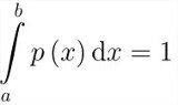
Now we generate 10 kilo-events using our method and build a histogram, simultaneously comparing it with the required probability density .
.
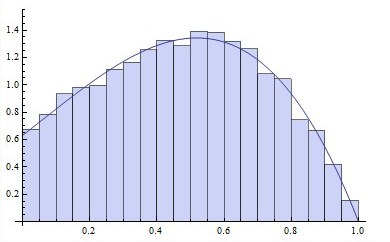
As you can see, the result exceeds all expectations! The effectiveness of this approach is the probability that the random value obtained using a set of standard random numbers ( ,
,  , ...,
  ) will be accepted, not discarded. For the Neumann method, it is easy to find that
We now turn to the final part of this article and see how MMK works in the FEC. To do this, we will not get into the wilds, but we will model the process of scattering a gamma-quantum on an electron that is known to everyone from school. In order not to reinvent the wheel, we’ll visit CERN, or rather in the Geant4 section, without any embarrassment, write off the Butler’s decomposition in the physics manual (yes, yes, the one I’m missing) and add formulas for calculating the secondary cosines and angles particles in lsk . I will not give calculations and do copy-paste because everything will be in the algorithm.
The differential cross section of this process is described by the Klein-Nishina formula - this is exactly the density of probabilities that we need:

We will conduct 10 kilo-events and construct the energy and angular distributions of secondary particles for the values of two energies 0.5 and 1.5 MeV, respectively.


How we can estimate on fingers, everything is very well considered and corresponds to the kinematics of the process, and therefore the method is very good.
It turns out that everything is simple enough, the main thing is to figure it out. I would like to tell you more, but I think a large amount will only bore anyone who is interested, I think they will look for literature - it’s great written in the manual I pulled from CERN, and even better from our teachers in the books. All calculations were performed in the natural calculus system and laboratory coordinate system.
Used Wolfram Mathematica 9.0
Immediately, I note that the simulation will be performed in the CAB WM , which I applied (not so long ago) in my first article.
Discrete random variables
Let's talk a little about probability theory and mathematical statistics using the example of a two-dice model. So, we are faced with the task of playing a typical situation at a casino playing table: “Play a certain number of events of simultaneously throwing two dice with numbers. According to the results of the draw, find the number of simultaneous hits of the numbers 2 and 4 ". In addition, we still burden ourselves with exception handling, so that this simple program has a zest.
Throwing 2 dice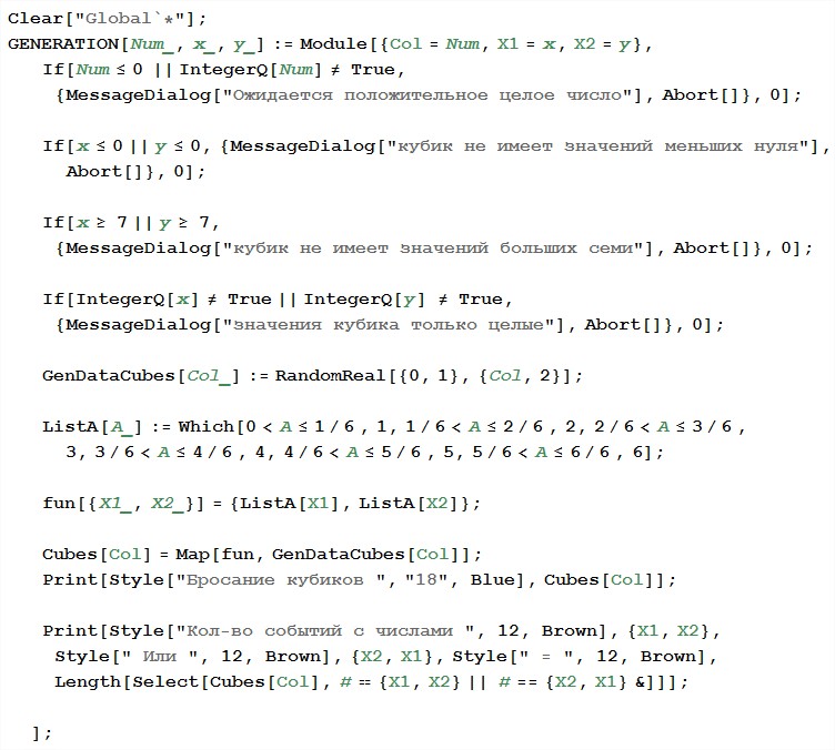
As we can see, everything is quite transparent, and the main part of the code is occupied by these same exams ... Let's look at the result of the program:
Klats
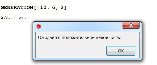
Note that the "triple" loss of 2 and 4 per sample of 10 events is an exclusive case, with a very small probability.
Thus, we played a pseudo-random discrete value by means of WM according to the algorithm given below.
Algorithm
- It is necessary to divide the interval (0,1) into n - intervals whose lengths are equal
 respectively.
 - Playing the value of a standard random variable
 (Standard PRNG ).
 - Checking the condition of hitting values in the i-th interval, long
 :
:  .
.
If the inequality is true, then we assign to the random variable χ the value corresponding to the given interval ie
- If necessary, repeat steps 1–3 several times using new values of the standard value γ to obtain other values of a discrete random variable with a law of probability distribution.
Neumann Method
Next we turn to playing out continuous random variables with the required probability density, as promised, by the Neumann method. In addition to the method of Neumann, there are also methods of superposition and inverse function, but the story about them is not the purpose of the article. And so, we set ourselves the next task: “Using the Neumann method, play a random variable with a distribution density:
on the interval x (0,1) ".Usually, physicists do not automate such things, but calculate everything in advance, then simply drive them through the cycle and get a sample. I, as a 21st century physicist, having powerful computer algebra systems in my arsenal, tried to automate the process. Let's see what came of it.
Neyman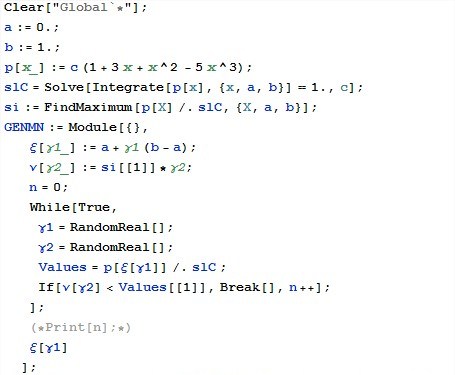
We see that everything is quite simple, just like in the book. The only thing that I would like to note is that for monotonically increasing or decreasing functions, which may be the required probability density type of quark-antiquaque anihilation, it is unlikely that we can find the search for the optimal value for the Neumann constant without exceptions. the values at the ends of the segments will always increase, which will be marked by WM warnings and, as a result, it will not be possible to embed it in the program block. The normalization constant with is calculated from the condition
Neumann's algorithm
This method is based on the following theorem from mathematical statistics and probability theory. Let be  -random value, with distribution density p (x) ≤ c ( c is some positive number) on the interval a <x <b, then if and - independent random variables and
  ,
,  then a random variable determined by the condition:
  , if a
  and has a probability density of p (x).
-random value, with distribution density p (x) ≤ c ( c is some positive number) on the interval a <x <b, then if and - independent random variables and , then a random variable determined by the condition: , if a and has a probability density of p (x).- We get a couple of values , with the help of PRNG.
- With their help, we build two random numbers uniformly distributed on the interval (a, b) and uniformly distributed on the interval (0, c)
- Using the constructed numbers, we check the condition
- If the condition is satisfied, then we assume that the value of a random variable equally
 if the condition is not met
then repeat the procedure from step 1.
Now we generate 10 kilo-events using our method and build a histogram, simultaneously comparing it with the required probability density
.As you can see, the result exceeds all expectations! The effectiveness of this approach is the probability that the random value obtained using a set of standard random numbers (
, , ..., ) will be accepted, not discarded. For the Neumann method, it is easy to find that Compton scattering of photons
We now turn to the final part of this article and see how MMK works in the FEC. To do this, we will not get into the wilds, but we will model the process of scattering a gamma-quantum on an electron that is known to everyone from school. In order not to reinvent the wheel, we’ll visit CERN, or rather in the Geant4 section, without any embarrassment, write off the Butler’s decomposition in the physics manual (yes, yes, the one I’m missing) and add formulas for calculating the secondary cosines and angles particles in lsk . I will not give calculations and do copy-paste because everything will be in the algorithm.
Compton scattering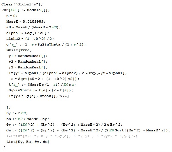
The differential cross section of this process is described by the Klein-Nishina formula - this is exactly the density of probabilities that we need:
We will conduct 10 kilo-events and construct the energy and angular distributions of secondary particles for the values of two energies 0.5 and 1.5 MeV, respectively.
How we can estimate on fingers, everything is very well considered and corresponds to the kinematics of the process, and therefore the method is very good.
Conclusion
It turns out that everything is simple enough, the main thing is to figure it out. I would like to tell you more, but I think a large amount will only bore anyone who is interested, I think they will look for literature - it’s great written in the manual I pulled from CERN, and even better from our teachers in the books. All calculations were performed in the natural calculus system and laboratory coordinate system.
Literature
- geant4.web.cern.ch/geant4/G4UsersDocuments/UsersGuides/PhysicsReferenceManual/html/PhysicsReferenceManual.html
- Andreev, V. V. “The Monte Carlo method in particle physics”. Curriculum special course, 2005. - 15 p.
Links
Used Wolfram Mathematica 9.0
')
Source: https://habr.com/ru/post/208666/
All Articles