We calculate what year is now from the Big Bang on Python
In connection with the coming year 2014 from the birth of Christ, the question may arise: “And what is actually the year now without being tied to religions?” I will try to answer it, or rather, show how it can be calculated quite easily without dismounting from the chair.
We will count from the beginning of the Universe, that is, the Big Bang. I will omit many reservations to get the result in the minimum number of formulas and lines of code (yes, we will program in Python!). As a bonus, we also estimate how much dark energy we have in the Universe.
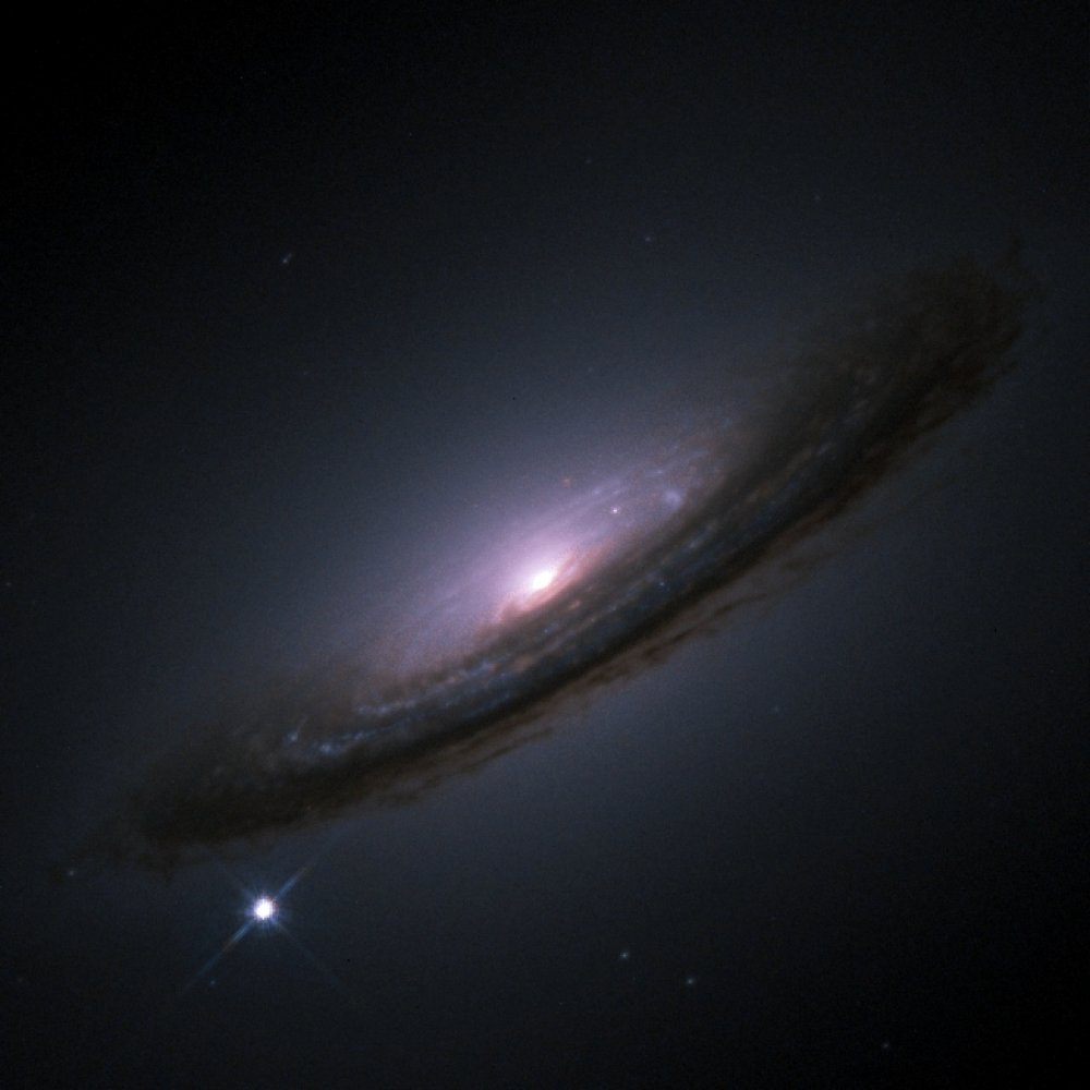
Supernova 1994D as seen with the Hubble Space Telescope. Foto: Pete Chalis - Harvard Smithsonian Center of Astrophysics
')
Curious? Then let's go!
Have you heard about Hubble? There is also a telescope named after him. So he discovered the fact that the Universe is increasing in size, or rather, the galaxies nearby, run away, and the farther they are from us, the faster they move away. How can the universe grow? The analogy may be simple. Imagine yourself an ant on a balloon inflated. It will seem to you that the world is slowly increasing, and the other ants on the ball are farther and farther away, although nothing happens to your body.
Returning to Hubble. How did he establish this fact? There are two points:
By measuring the speed with which the Universe is increasing, we can estimate when it was a point. This moment can be called the beginning of everything and estimate how many years ago it was.
We will need Python (the version is unimportant, I will use 2.7, the differences from 3. * are minimal):
For calculations we will use Numpy and Scipy :
And for Matplotlib charts:
For gentlemen without root, I recommend this build: store.continuum.io/cshop/anaconda
For Windows users: code.google.com/p/pythonxy
We believe that the system prepared. Everything that goes further can be run online (right in the Python console), or in iPython. As you like.
The beauty of modern astrophysics in the complete openness of observational data. We will use this catalog of type Ia supernovae, which I wrote about above: supernova.lbl.gov/Union
We will need this file: supernova.lbl.gov/Union/figures/SCPUnion2.1_mu_vs_z.txt
Let's connect libraries which will be required later.
Load the data from the file and create three auxiliary arrays:
The fact that such a distance modulus and how to get the distance from an object from it is succinctly written on the Belarusian Wikipedia .
We convert this quantity, the existence of which is caused solely by the convenience of observers, into a physical one. The distance to the object is written in the array DL :
When calculating Distance Modulus, the authors of the catalog suggested that the luminosity of the supernova is -19.3, as described in the description. They did this work for us.
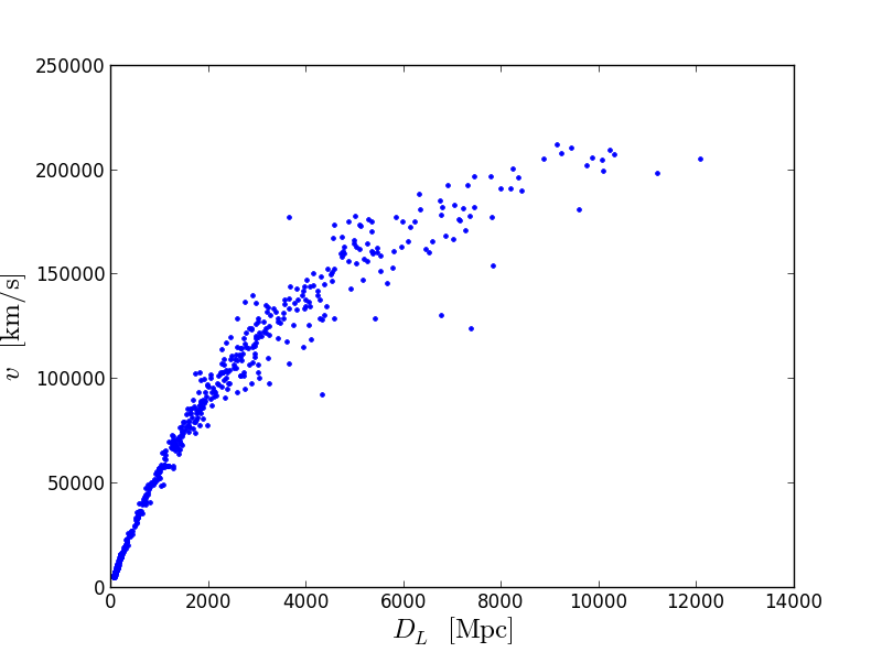
Now in the variable z we have redshifts and in DL - distances in Megaparsecs (1 parse = 3e16 meters = 3.3 light years). You can build a picture and see what happened:

Now let's convert the redshift, z , to speed. To begin, we need a function to convert the speed into a redshift, that is, the inverse function:
The formula is taken from here: en.wikipedia.org/wiki/Redshift#Redshift_formulae
To convert in the opposite direction, we will calculate in advance the correspondence between z_list and v_list, after which we will write a function that interpolates between points:
Let's look at the speed of an object depending on its distance from us:
This picture clearly shows that the farther the object, the faster it moves away from us. Let's try to profit direct. The slope of the straight line (derivative) at point 0 is called the Hubble constant, H , and is measured in km / s / Mps. You can find this slope by fitting, but we will go in a simple way. Just pick the slope:
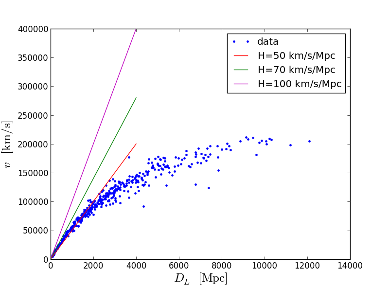
And an enlarged version:
The most accurate guess: H = 70 km / s / Mps. That is, the object located in 1 Mps away from us at a speed of 70 km / s. In other words, we were with him at one point so many years ago (assuming that the speed of divergence was constant):
(1 Mps) / (70 km / s) = 1 / H = 14,000,000,000 years ago
( Google is good at converting various units of measurement.)
So, after a few lines of code, we found that the age of the universe is about 14 billion years. First, it is a very rough estimate. Secondly, we did not appreciate the measurement error, which must be done in any experiment. We also did not say how we know the brightness of supernova explosions, and why we consider them the same. These are also separate interesting topics. Nevertheless, such a rough estimate gives a good result! A more accurate analysis with all known observations gives a result of 13.813 ± 0.058 billion years.
At the time, Hubble observed only the very beginning of such a diagram (from his 1929 article apod.nasa.gov/diamond_jubilee/d_1996/hub_1929.html )

and received instead of 70, the number 500. However, the error is less than 10 times, which is defended for hit.
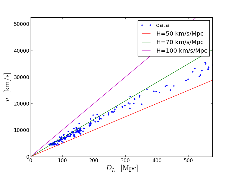
In the figures you can see that the line fits only at the beginning of the diagram. Further, the linear approximation does not fit at all. For the next step, we will need to dive a bit into cosmology. In the simplest model, the Universe consists of matter and of dark energy (Einstein's lambda term), and at the same time is flat. Having designated the part of the Universe, consisting of matter, for Omega_M and another part of the Universe of some dark energy, for Omega_L, and Omega_M + Omega_L = 1, I can express the distance to an object through redshift using the formula (you can read more on Wikipedia: [1] [2] ):
Introduce the auxiliary function E (z):

Omega_k, which appears here, is responsible for the curvature of the universe. For simplicity, we consider it flat, that is, Omega_k = 0. Therefore, in the following formula, we need a middle line:
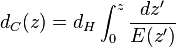
Key integral
Additional factor (1 + z), the origin of which is too long to explain :):

Next, write the code that calculates the integral:
The green curve fits the data a little better. For the sake of simplicity, we forget about the error of fitting the theory into the data. The conclusion is the following. The amount of dark energy and matter are comparable today (models in which the ratio of 100 to 1 does not fit into the data). This is quite an interesting fact. About ~ 70% of the Universe is some kind of dark energy, the nature of which we do not understand yet. The remaining ~ 30% of matter is also not as simple as it seems. From it only the fifth part is baryonic matter (that of which we consist), and the rest is dark matter . As for it, its amount can also be estimated some other time.
Well, here we are. Lastly, I’ll just say that this is far from the only way to measure the geometry and age of the Universe. There are several of them. And remarkably, they all speak in favor of the theory of the Big Bang and the expanding Universe.
Happy celebration of the name day of Jesus, gentlemen! :)
We will count from the beginning of the Universe, that is, the Big Bang. I will omit many reservations to get the result in the minimum number of formulas and lines of code (yes, we will program in Python!). As a bonus, we also estimate how much dark energy we have in the Universe.
Supernova 1994D as seen with the Hubble Space Telescope. Foto: Pete Chalis - Harvard Smithsonian Center of Astrophysics
')
Curious? Then let's go!
Briefly about the physical side of the issue
Have you heard about Hubble? There is also a telescope named after him. So he discovered the fact that the Universe is increasing in size, or rather, the galaxies nearby, run away, and the farther they are from us, the faster they move away. How can the universe grow? The analogy may be simple. Imagine yourself an ant on a balloon inflated. It will seem to you that the world is slowly increasing, and the other ants on the ball are farther and farther away, although nothing happens to your body.
Returning to Hubble. How did he establish this fact? There are two points:
- First, we must measure the speed of the galaxy. Here we need the Doppler effect. We all know about the classic experiment with the whistle of the train at the moment when it sweeps along the apron. When an object moves away from us, the wavelength it radiates is extended. From this amendment, you can find the speed. In astronomy, this increase is called the redshift and denoted by the letter z . Some known spectral line is observed and, finding its displacement, they calculate the speed.
- Secondly, the distance to the galaxy. Just because the distance to them is not measured. Here we will need an additional object - type Ia supernovae. These are the explosions of stars, in which the same amount of energy is released. For the brightness that we observe, you can calculate the distance to the explosion itself and to the galaxy in which this explosion occurred. Pictured above is a galaxy and a supernova explosion. In terms of brightness, it surpasses the entire galaxy, in which about a hundred billion stars.
And where is the age of the universe?
By measuring the speed with which the Universe is increasing, we can estimate when it was a point. This moment can be called the beginning of everything and estimate how many years ago it was.
Prepare the system
We will need Python (the version is unimportant, I will use 2.7, the differences from 3. * are minimal):
sudo apt-get install pythonFor calculations we will use Numpy and Scipy :
pip install numpypip install scipyAnd for Matplotlib charts:
pip install matplotlibFor gentlemen without root, I recommend this build: store.continuum.io/cshop/anaconda
For Windows users: code.google.com/p/pythonxy
We believe that the system prepared. Everything that goes further can be run online (right in the Python console), or in iPython. As you like.
Download data
The beauty of modern astrophysics in the complete openness of observational data. We will use this catalog of type Ia supernovae, which I wrote about above: supernova.lbl.gov/Union
We will need this file: supernova.lbl.gov/Union/figures/SCPUnion2.1_mu_vs_z.txt
Start writing code
Let's connect libraries which will be required later.
import numpy as np import matplotlib.pyplot as plt Load the data from the file and create three auxiliary arrays:
# 5 , . # 0 , , data=np.loadtxt('SCPUnion2.1_mu_vs_z.txt',skiprows=5,converters={0: lambda s: 0}) # z = data[:,1] # distance modulus DM = data[:,2] DM_err=data[:,3] The fact that such a distance modulus and how to get the distance from an object from it is succinctly written on the Belarusian Wikipedia .
We convert this quantity, the existence of which is caused solely by the convenience of observers, into a physical one. The distance to the object is written in the array DL :
# def DM2DL(DM): return 10**(DM/5-1)/1e4 # DL=DM2DL(DM) When calculating Distance Modulus, the authors of the catalog suggested that the luminosity of the supernova is -19.3, as described in the description. They did this work for us.
Now in the variable z we have redshifts and in DL - distances in Megaparsecs (1 parse = 3e16 meters = 3.3 light years). You can build a picture and see what happened:
plt.plot(DL,z,'.') plt.xlabel(r'$D_{L}\;\mathrm{[Mpc]}$',size=18) plt.ylabel(r'$z$',size=18) Now let's convert the redshift, z , to speed. To begin, we need a function to convert the speed into a redshift, that is, the inverse function:
# # c=29979245800 # cm/s # def v2z(v): return sqrt((1.0+v/c)/(1.0-v/c))-1.0 The formula is taken from here: en.wikipedia.org/wiki/Redshift#Redshift_formulae
To convert in the opposite direction, we will calculate in advance the correspondence between z_list and v_list, after which we will write a function that interpolates between points:
v_list=linspace(0,c,100) z_list=v2z(v_list) # plt.plot(z_list,v_list) def z2v(z): return np.interp(z,z_list,v_list)/1e5 v=z2v(z) # km/s Let's look at the speed of an object depending on its distance from us:
plt.plot(DL,v,'.') plt.xlabel(r'$D_{L}\;\mathrm{[Mpc]}$',size=18) plt.ylabel(r'$v\;\mathrm{[km/s]}$',size=18) This picture clearly shows that the farther the object, the faster it moves away from us. Let's try to profit direct. The slope of the straight line (derivative) at point 0 is called the Hubble constant, H , and is measured in km / s / Mps. You can find this slope by fitting, but we will go in a simple way. Just pick the slope:
plt.plot(DL,v,'.') plt.xlabel(r'$D_{L}\;\mathrm{[Mpc]}$',size=18) plt.ylabel(r'$v\;\mathrm{[km/s]}$',size=18) temp=np.array([0.0,20.0]) plt.plot(temp,50.0*temp,'r') plt.plot(temp,70.0*temp,'g') plt.plot(temp,100.0*temp,'m') plt.legend(('data','H=50','H=70','H=100')) And an enlarged version:
The most accurate guess: H = 70 km / s / Mps. That is, the object located in 1 Mps away from us at a speed of 70 km / s. In other words, we were with him at one point so many years ago (assuming that the speed of divergence was constant):
(1 Mps) / (70 km / s) = 1 / H = 14,000,000,000 years ago
( Google is good at converting various units of measurement.)
So, after a few lines of code, we found that the age of the universe is about 14 billion years. First, it is a very rough estimate. Secondly, we did not appreciate the measurement error, which must be done in any experiment. We also did not say how we know the brightness of supernova explosions, and why we consider them the same. These are also separate interesting topics. Nevertheless, such a rough estimate gives a good result! A more accurate analysis with all known observations gives a result of 13.813 ± 0.058 billion years.
At the time, Hubble observed only the very beginning of such a diagram (from his 1929 article apod.nasa.gov/diamond_jubilee/d_1996/hub_1929.html )
and received instead of 70, the number 500. However, the error is less than 10 times, which is defended for hit.
Dark energy?
In the figures you can see that the line fits only at the beginning of the diagram. Further, the linear approximation does not fit at all. For the next step, we will need to dive a bit into cosmology. In the simplest model, the Universe consists of matter and of dark energy (Einstein's lambda term), and at the same time is flat. Having designated the part of the Universe, consisting of matter, for Omega_M and another part of the Universe of some dark energy, for Omega_L, and Omega_M + Omega_L = 1, I can express the distance to an object through redshift using the formula (you can read more on Wikipedia: [1] [2] ):
Introduce the auxiliary function E (z):
Omega_k, which appears here, is responsible for the curvature of the universe. For simplicity, we consider it flat, that is, Omega_k = 0. Therefore, in the following formula, we need a middle line:
Key integral
Additional factor (1 + z), the origin of which is too long to explain :):
Next, write the code that calculates the integral:
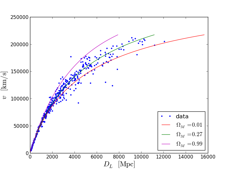
# E_z def e_Z(z, OmegaM): OmegaL=1.0-OmegaM return (OmegaM*(1.0+z)**3+OmegaL)**(-0.5) # scipy import scipy.integrate as si # def D_L(z, OmegaM): dh=4286.0 # c/H, H 70 // D_c=dh*si.quad(e_Z,0.0,z,args=(OmegaM))[0] return D_c*(1.0+z) # , def D_L_batch(z,OmegaM,H): DL=z.copy() for i in range(len(z)): DL[i]=D_L(z[i],OmegaM,H) return DL # plt.plot(DL,v,'.') plt.xlabel(r'$D_{L}\;\mathrm{[Mpc]}$',size=18) plt.ylabel(r'$v\;\mathrm{[km/s]}$',size=18) # z- 0 1.5, 100 temp_z=np.linspace(0,1.5,100) # v- temp_v=z2v(temp_z) # Omega_M plt.plot(D_L_batch(temp_z,0.01,70.0),temp_v,'r') plt.plot(D_L_batch(temp_z,0.27,70.0),temp_v,'g') plt.plot(D_L_batch(temp_z,0.99,70.0),temp_v,'m') plt.legend(('data',r'$\Omega_M=0.01$',r'$\Omega_M=0.27$',r'$\Omega_M=0.99$'),loc=4) The green curve fits the data a little better. For the sake of simplicity, we forget about the error of fitting the theory into the data. The conclusion is the following. The amount of dark energy and matter are comparable today (models in which the ratio of 100 to 1 does not fit into the data). This is quite an interesting fact. About ~ 70% of the Universe is some kind of dark energy, the nature of which we do not understand yet. The remaining ~ 30% of matter is also not as simple as it seems. From it only the fifth part is baryonic matter (that of which we consist), and the rest is dark matter . As for it, its amount can also be estimated some other time.
Well, here we are. Lastly, I’ll just say that this is far from the only way to measure the geometry and age of the Universe. There are several of them. And remarkably, they all speak in favor of the theory of the Big Bang and the expanding Universe.
Happy celebration of the name day of Jesus, gentlemen! :)
Source: https://habr.com/ru/post/207822/
All Articles