Time Series Analysis with Python
Good afternoon, dear readers.
In today's article, I will try to describe the process of analyzing time series using python and the statsmodels module. This module provides a wide range of tools and methods for statistical analysis and econometrics. I will try to show the main stages of the analysis of such series, in conclusion, we will build the ARIMA model.
For example, we took real data on the turnover of one of the warehouse complexes in the Moscow region.
First, load the data and take a look at it:
So, as you can see the read_csv () function, in this case, in addition to specifying the parameters that define the columns and index used, you can notice 3 more parameters for working with the date. Let us dwell on them in more detail.
parse_dates specifies the column names to be converted to a DateTime type. It is worth noting that if there are empty values in this column, the parsing will fail and the object type column will return. To avoid this, you must add the keep_default_na = False parameter.
The final parameter dayfirst indicates the parsing function that the first in the line is the first day, not vice versa. If you do not set this parameter, the function may not correctly convert dates and confuse the month and day in some places. For example, 01/02/2013 will be converted to 02-01-2013 , which will be wrong.
Let's separate in a separate series a time series with values of shipments:
')
So, we now have a time series and we can proceed to its analysis.
To begin, let's look at the schedule for our series:
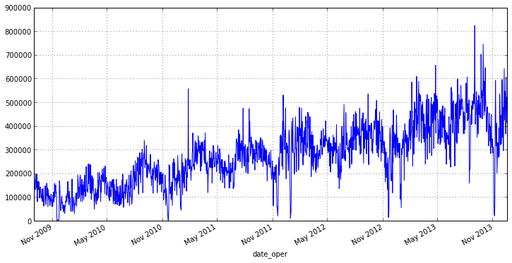
From the graph it is clear that our series has a small amount of emissions that affect the scatter. In addition, analyzing shipments for each day is not quite true, since, for example, at the end or beginning of the week there will be days in which the goods are shipped much more than the rest. Therefore, it makes sense to go to the weekly interval and the average value of shipments on it, it will save us from emissions and reduce the fluctuations of our series. In pandas, for this there is a convenient function resample () , as parameters it is passed the rounding period and the aggregate function:
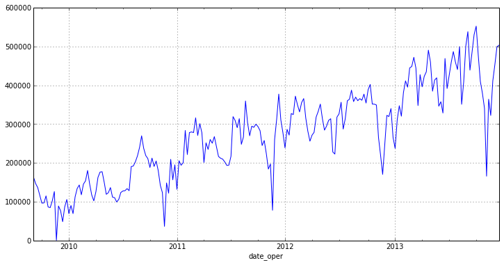
As you can see, the new chart has no bright emissions and has a pronounced trend. From this we can conclude that the series is not stationary [1] .
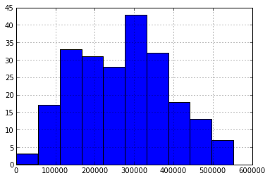
As can be seen from the characteristics and the histogram, the series is more or less homogeneous and has a relatively small variation, as evidenced by the coefficient of variation : where
where  - standard deviation ,
  - arithmetic average of the sample. In our case, it is equal to:
V = 0.437022
We will carry out the Harkey -Bera test to determine the nominal distribution, to confirm the assumption of homogeneity. To do this, there is a function jarque_bera () , which returns the values of these statistics:
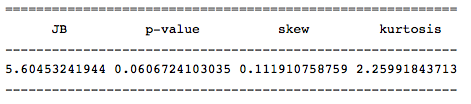
The value of this statistic indicates that the null hypothesis of normal distribution is rejected with a small probability ( probably> 0.05 ), and, therefore, our series has a normal distribution.
The SimpleTable () function serves to format the output. In our case, the input to it is an array of values (dimensionality not greater than 2) and a list with the names of columns or rows.
Many methods and models are based on assumptions about the stationarity of a series, but as noted earlier, our series most likely is not. Therefore, to test the stationarity test, let's conduct a generalized Dickey-Fuller test for the presence of unit roots. For this, the statsmodels module has the adfuller () function:
adf: -1.38835541357
p-value: 0.58784577297
Critical values: {'5%': -2.8753374677799957, '1%': -3.4617274344627398, '10% ': -2.5741240890815571}
there are single roots, the series is not stationary
The test confirmed the assumptions about the non-stationarity of the series. In many cases, taking the difference of rows allows this. If, for example, the first differences of a row are stationary, then it is called an integrated series of the first order .
So let's define the order of the integrated series for our series:
In the above code, the diff () function calculates the difference of the original series with the specified period offset. The offset period is passed as the period parameter. Since in difference the first value is vague, then we need to get rid of it for this and use the dropna () method.
Check the resulting series for stationarity:
adf: -5.95204224907
p-value: 2.13583392404e-07
Critical values: {'5%': -2.8755379867788462, '1%': -3.4621857592784546, '10% ': -2.574231080806213}
there are no unit roots, the row is stationary
As can be seen from the code above, the resulting series of first differences approached the stationary one. For complete confidence, we divide it into several intervals and verify the mat. expectations at different intervals:
p-value: 0.693072039563
A high p-value gives us the opportunity to argue that the null hypothesis of equality of averages is correct, which indicates the stationarity of the series. It remains to make sure that there is no trend for this. Let's build a graph of our new series:

The trend is really absent, so the series of first differences is stationary, and our initial series is an integrated series of the first order .
For the simulation, we will use the ARIMA model, built for a number of first differences.
So, to build a model, we need to know its order, consisting of 2 parameters:
The parameter d is and it is equal to 1, it remains to determine p and q . To determine them, we need to study the autocorrelation (ACF) and partially autocorrelation (PACF) functions for a number of first differences.
ACF will help us determine q , because by its correlogram you can determine the number of autocorrelation coefficients that are very different from 0 in the MA model
PACF will help us determine p , because from its correlogram you can determine the maximum coefficient number that is very different from 0 in the AR model.
To construct the corresponding correlograms, the following functions are included in the statsmodels package: plot_acf () and plot_pacf () . They display ACF and PACF plots , in which the lag numbers are plotted along the X axis, and the values of the corresponding functions along the Y axis. It should be noted that the number of lags in functions determines the number of significant coefficients. So, our functions look like this:
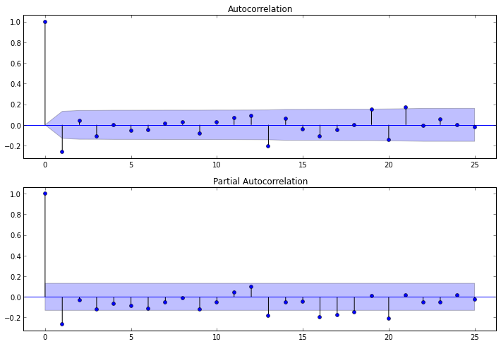
After studying the PACF correlogram, we can conclude that p = 1 , since on it only 1 lag is very different from zero. According to the ACF correlogram, you can see that q = 1 , since after lag 1, the values of the functions fall sharply.
So, when all the parameters are known, you can build a model, but to build it, we will not take all the data, but only a part. We will leave the data from the parts not included in the model to check the accuracy of the forecast of our model:
The trend parameter is responsible for the presence of a constant in the model. Let's display information on the resulting model:
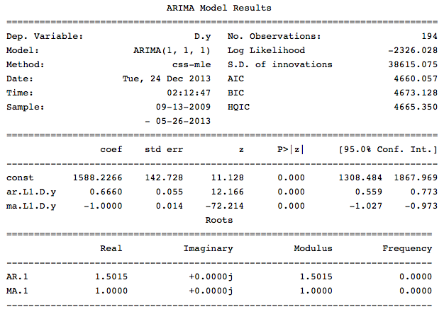
As can be seen from this information in our model, all the coefficients are significant and you can proceed to the evaluation of the model.
We will check the residuals of this model for compliance with “white noise” , and also analyze the residual correlogram, as this can help us in determining the regression elements important for inclusion and prediction.
So the first thing we will do is conduct a Ljung-Box Q test to test the hypothesis that the residues are random, that is, they are “white noise”. This test is conducted on the remnants of the model ARIMA . Thus, we need to first obtain the remnants of the model and build an ACF for them, and then mark the test for the resulting coefficients. With the help of statsmadels you can do it like this:
The value of these statistics and p-values indicate that the hypothesis of randomness of residuals is not rejected, and most likely this process represents “white noise”.
Now let's calculate the coefficient of determination To understand what percentage of observations this model describes:
R ^ 2: -0.03
The standard deviation [2] of our model:
80919.057367642512
Mean absolute error [2] of the forecast:
63092.763277651895
It remains to draw our forecast on the chart:
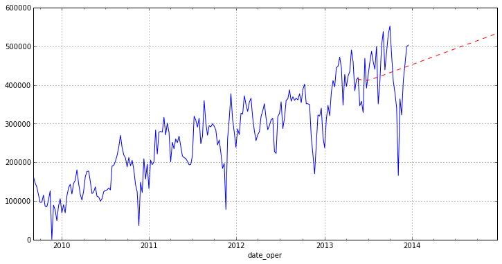
As you can see from the graph, our model is not building a very good forecast. This is partly due to emissions in the original data that we have not completely removed, as well as the ARIMA module of the statsmodels package, since it is fairly new. The article is more aimed at showing how exactly you can analyze time series in python. I would also like to note that in the package reviewed today, various methods of regression analysis are very fully implemented (I will try to show in further articles).
In general, the statsmodels package is fully suitable for small studies, but for serious scientific work it is still damp and some tests and statistics are missing in it.
In today's article, I will try to describe the process of analyzing time series using python and the statsmodels module. This module provides a wide range of tools and methods for statistical analysis and econometrics. I will try to show the main stages of the analysis of such series, in conclusion, we will build the ARIMA model.
For example, we took real data on the turnover of one of the warehouse complexes in the Moscow region.
Loading and preliminary data processing
First, load the data and take a look at it:
from pandas import read_csv, DataFrame import statsmodels.api as sm from statsmodels.iolib.table import SimpleTable from sklearn.metrics import r2_score import ml_metrics as metrics In [2]: dataset = read_csv('tovar_moving.csv',';', index_col=['date_oper'], parse_dates=['date_oper'], dayfirst=True) dataset.head() | Otgruzka | priemka | |
|---|---|---|
| date_oper | ||
| 2009-09-01 | 179667 | 276712 |
| 2009-09-02 | 177670 | 164999 |
| 2009-09-03 | 152112 | 189181 |
| 2009-09-04 | 142938 | 254581 |
| 2009-09-05 | 130741 | 192486 |
So, as you can see the read_csv () function, in this case, in addition to specifying the parameters that define the columns and index used, you can notice 3 more parameters for working with the date. Let us dwell on them in more detail.
parse_dates specifies the column names to be converted to a DateTime type. It is worth noting that if there are empty values in this column, the parsing will fail and the object type column will return. To avoid this, you must add the keep_default_na = False parameter.
The final parameter dayfirst indicates the parsing function that the first in the line is the first day, not vice versa. If you do not set this parameter, the function may not correctly convert dates and confuse the month and day in some places. For example, 01/02/2013 will be converted to 02-01-2013 , which will be wrong.
Let's separate in a separate series a time series with values of shipments:
')
otg = dataset.Otgruzka otg.head() | date_oper | |
| 2009-09-01 | 179667 |
| 2009-09-02 | 177670 |
| 2009-09-03 | 152112 |
| 2009-09-04 | 142938 |
| 2009-09-05 | 130741 |
| Name: Otgruzka, dtype: int64 | |
So, we now have a time series and we can proceed to its analysis.
Time series analysis
To begin, let's look at the schedule for our series:
otg.plot(figsize=(12,6)) From the graph it is clear that our series has a small amount of emissions that affect the scatter. In addition, analyzing shipments for each day is not quite true, since, for example, at the end or beginning of the week there will be days in which the goods are shipped much more than the rest. Therefore, it makes sense to go to the weekly interval and the average value of shipments on it, it will save us from emissions and reduce the fluctuations of our series. In pandas, for this there is a convenient function resample () , as parameters it is passed the rounding period and the aggregate function:
otg = otg.resample('W', how='mean') otg.plot(figsize=(12,6)) As you can see, the new chart has no bright emissions and has a pronounced trend. From this we can conclude that the series is not stationary [1] .
itog = otg.describe() otg.hist() itog | count | 225 |
| mean | 270858.285365 |
| std | 118371.082975 |
| min | 872.857143 |
| 25% | 180263.428571 |
| 50% | 277898.714286 |
| 75% | 355587.285714 |
| max | 552485.142857 |
| dtype: float64 | |
As can be seen from the characteristics and the histogram, the series is more or less homogeneous and has a relatively small variation, as evidenced by the coefficient of variation :
where - standard deviation , - arithmetic average of the sample. In our case, it is equal to: print 'V = %f' % (itog['std']/itog['mean']) V = 0.437022
We will carry out the Harkey -Bera test to determine the nominal distribution, to confirm the assumption of homogeneity. To do this, there is a function jarque_bera () , which returns the values of these statistics:
row = [u'JB', u'p-value', u'skew', u'kurtosis'] jb_test = sm.stats.stattools.jarque_bera(otg) a = np.vstack([jb_test]) itog = SimpleTable(a, row) print itog The value of this statistic indicates that the null hypothesis of normal distribution is rejected with a small probability ( probably> 0.05 ), and, therefore, our series has a normal distribution.
The SimpleTable () function serves to format the output. In our case, the input to it is an array of values (dimensionality not greater than 2) and a list with the names of columns or rows.
Many methods and models are based on assumptions about the stationarity of a series, but as noted earlier, our series most likely is not. Therefore, to test the stationarity test, let's conduct a generalized Dickey-Fuller test for the presence of unit roots. For this, the statsmodels module has the adfuller () function:
test = sm.tsa.adfuller(otg) print 'adf: ', test[0] print 'p-value: ', test[1] print'Critical values: ', test[4] if test[0]> test[4]['5%']: print ' , ' else: print ' , ' adf: -1.38835541357
p-value: 0.58784577297
Critical values: {'5%': -2.8753374677799957, '1%': -3.4617274344627398, '10% ': -2.5741240890815571}
there are single roots, the series is not stationary
The test confirmed the assumptions about the non-stationarity of the series. In many cases, taking the difference of rows allows this. If, for example, the first differences of a row are stationary, then it is called an integrated series of the first order .
So let's define the order of the integrated series for our series:
otg1diff = otg.diff(periods=1).dropna() In the above code, the diff () function calculates the difference of the original series with the specified period offset. The offset period is passed as the period parameter. Since in difference the first value is vague, then we need to get rid of it for this and use the dropna () method.
Check the resulting series for stationarity:
test = sm.tsa.adfuller(otg1diff) print 'adf: ', test[0] print 'p-value: ', test[1] print'Critical values: ', test[4] if test[0]> test[4]['5%']: print ' , ' else: print ' , ' adf: -5.95204224907
p-value: 2.13583392404e-07
Critical values: {'5%': -2.8755379867788462, '1%': -3.4621857592784546, '10% ': -2.574231080806213}
there are no unit roots, the row is stationary
As can be seen from the code above, the resulting series of first differences approached the stationary one. For complete confidence, we divide it into several intervals and verify the mat. expectations at different intervals:
m = otg1diff.index[len(otg1diff.index)/2+1] r1 = sm.stats.DescrStatsW(otg1diff[m:]) r2 = sm.stats.DescrStatsW(otg1diff[:m]) print 'p-value: ', sm.stats.CompareMeans(r1,r2).ttest_ind()[1] p-value: 0.693072039563
A high p-value gives us the opportunity to argue that the null hypothesis of equality of averages is correct, which indicates the stationarity of the series. It remains to make sure that there is no trend for this. Let's build a graph of our new series:
otg1diff.plot(figsize=(12,6)) The trend is really absent, so the series of first differences is stationary, and our initial series is an integrated series of the first order .
Building a time series model
For the simulation, we will use the ARIMA model, built for a number of first differences.
So, to build a model, we need to know its order, consisting of 2 parameters:
The parameter d is and it is equal to 1, it remains to determine p and q . To determine them, we need to study the autocorrelation (ACF) and partially autocorrelation (PACF) functions for a number of first differences.
ACF will help us determine q , because by its correlogram you can determine the number of autocorrelation coefficients that are very different from 0 in the MA model
PACF will help us determine p , because from its correlogram you can determine the maximum coefficient number that is very different from 0 in the AR model.
To construct the corresponding correlograms, the following functions are included in the statsmodels package: plot_acf () and plot_pacf () . They display ACF and PACF plots , in which the lag numbers are plotted along the X axis, and the values of the corresponding functions along the Y axis. It should be noted that the number of lags in functions determines the number of significant coefficients. So, our functions look like this:
ig = plt.figure(figsize=(12,8)) ax1 = fig.add_subplot(211) fig = sm.graphics.tsa.plot_acf(otg1diff.values.squeeze(), lags=25, ax=ax1) ax2 = fig.add_subplot(212) fig = sm.graphics.tsa.plot_pacf(otg1diff, lags=25, ax=ax2) After studying the PACF correlogram, we can conclude that p = 1 , since on it only 1 lag is very different from zero. According to the ACF correlogram, you can see that q = 1 , since after lag 1, the values of the functions fall sharply.
So, when all the parameters are known, you can build a model, but to build it, we will not take all the data, but only a part. We will leave the data from the parts not included in the model to check the accuracy of the forecast of our model:
src_data_model = otg[:'2013-05-26'] model = sm.tsa.ARIMA(src_data_model, order=(1,1,1), freq='W').fit(full_output=False, disp=0) The trend parameter is responsible for the presence of a constant in the model. Let's display information on the resulting model:
print model.summary() As can be seen from this information in our model, all the coefficients are significant and you can proceed to the evaluation of the model.
Model analysis and evaluation
We will check the residuals of this model for compliance with “white noise” , and also analyze the residual correlogram, as this can help us in determining the regression elements important for inclusion and prediction.
So the first thing we will do is conduct a Ljung-Box Q test to test the hypothesis that the residues are random, that is, they are “white noise”. This test is conducted on the remnants of the model ARIMA . Thus, we need to first obtain the remnants of the model and build an ACF for them, and then mark the test for the resulting coefficients. With the help of statsmadels you can do it like this:
q_test = sm.tsa.stattools.acf(model.resid, qstat=True) # resid, , qstat=True, - print DataFrame({'Q-stat':q_test[1], 'p-value':q_test[2]}) Result
| Q-stat | p-value | |
|---|---|---|
| 0 | 0.531426 | 0.466008 |
| one | 3.073217 | 0.215109 |
| 2 | 3.644229 | 0.302532 |
| 3 | 3.906326 | 0.418832 |
| four | 4.701433 | 0.453393 |
| five | 5.433745 | 0.489500 |
| 6 | 5.444254 | 0.605916 |
| 7 | 5.445309 | 0.709091 |
| eight | 5.900762 | 0.749808 |
| 9 | 6.004928 | 0.814849 |
| ten | 6.155966 | 0.862758 |
| eleven | 6.299958 | 0.900213 |
| 12 | 12.731542 | 0.468755 |
| 13 | 14.707894 | 0.398410 |
| 14 | 20.720607 | 0.145996 |
| 15 | 23.197433 | 0.108558 |
| sixteen | 23.949801 | 0.120805 |
| 17 | 24.119236 | 0.151160 |
| 18 | 25.616184 | 0.141243 |
| nineteen | 26.035165 | 0.164654 |
| 20 | 28.969880 | 0.114727 |
| 21 | 28.973660 | 0.145614 |
| 22 | 29.017716 | 0.179723 |
| 23 | 32.114006 | 0.124191 |
| 24 | 32.284805 | 0.149936 |
| 25 | 33.123395 | 0.158548 |
| 26 | 33.129059 | 0.192844 |
| 27 | 33.760488 | 0.208870 |
| 28 | 38.421053 | 0.113255 |
| 29 | 38.724226 | 0.132028 |
| thirty | 38.973426 | 0.153863 |
| 31 | 38.978172 | 0.184613 |
| 32 | 39.318954 | 0.207819 |
| 33 | 39.382472 | 0.241623 |
| 34 | 39.423763 | 0.278615 |
| 35 | 40.083689 | 0.293860 |
| 36 | 43.849515 | 0.203755 |
| 37 | 45.704476 | 0.182576 |
| 38 | 47.132911 | 0.174117 |
| 39 | 47.365305 | 0.197305 |
The value of these statistics and p-values indicate that the hypothesis of randomness of residuals is not rejected, and most likely this process represents “white noise”.
Now let's calculate the coefficient of determination
To understand what percentage of observations this model describes: pred = model.predict('2013-05-26','2014-12-31', typ='levels') trn = otg['2013-05-26':] r2 = r2_score(trn, pred[1:32]) print 'R^2: %1.2f' % r2 R ^ 2: -0.03
The standard deviation [2] of our model:
metrics.rmse(trn,pred[1:32]) 80919.057367642512
Mean absolute error [2] of the forecast:
metrics.mae(trn,pred[1:32]) 63092.763277651895
It remains to draw our forecast on the chart:
otg.plot(figsize=(12,6)) pred.plot(style='r--') Conclusion
As you can see from the graph, our model is not building a very good forecast. This is partly due to emissions in the original data that we have not completely removed, as well as the ARIMA module of the statsmodels package, since it is fairly new. The article is more aimed at showing how exactly you can analyze time series in python. I would also like to note that in the package reviewed today, various methods of regression analysis are very fully implemented (I will try to show in further articles).
In general, the statsmodels package is fully suitable for small studies, but for serious scientific work it is still damp and some tests and statistics are missing in it.
Links
- I.I. Eliseev. Econometrics
- Comparison of time series models
Source: https://habr.com/ru/post/207160/
All Articles