Constructing the Julia Set

Hey. Passions are raging, the end of the year, sessions, deadlines, the new year, as well as censorship penetrates into all layers of the Internet, which can not but grieve. Habr is no longer a cake . I just wanted to write that I do not agree with this approach, but then I would just be banned. So you have to write interesting content. Although if you are banned because of the preface to the post about Julia's set, well, then the remains of the cake have fallen out and there is no chance.

So back to the topic of the post. I have long wanted to learn a little more about complex numbers, and not just that the root of minus one is i. Particularly interesting were figures with a fractal structure, I wanted to understand what it means and how to make such visualization. Somewhere on the shelf was a book on the complex function of the complex , as well as a course on complex analysis on the cursor , and a little free time from work appeared. Let's get started

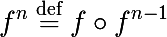
Function iteration

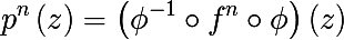
Before you write an algorithm, you will have to learn a few basic concepts. We begin with the concept of iterating the function f . We introduce the following notation for the nth iteration of the function f :

• where ○ is the composition of functions

The zero mapping is the identity mapping :

')
There are many theorems about fixed points of certain types of mappings; let us recall what a fixed point of some mapping g is , this is a solution to the following equation:


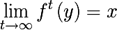
Similarly, for iterating a function, a attracting point is introduced — such a point from the domain of the function f , that the sequence value of the iterations of the function f converges to some fixed point of the map f :

• where y is some point close enough to the point x

The set of all y satisfying the previous condition is called the limit set of the point x under the action of iteration of the function f .

As a rule, it is of interest to study the sequence of functions formed by iterations (a similar idea can be seen in Newton's method , the desired solution turns out to be the attracting fixed point of the constructed map, and therefore can be found as the limit of the sequence of iterations.)



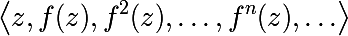
as well as a sequence of values ​​calculated at some starting point



For a complex world, visualizing the iterative convergence of the point y to x under the action of the iteration of the function f is a bit problematic, all the same 4d, but for the real world the picture is only 2d (the red path diverges while the blue converges to a fixed point).



So, the first pebble necessary for understanding the Julia set is laid, we proceed to the next.

Quadratic complex polynomial

In general, the Julia set is constructed for a function of the form

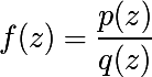
• where p and q are complex polynomials

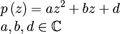
We will simplify the problem, and we will build the Julia set only for a quadratic polynomial. A quadratic complex polynomial in general form is as follows:



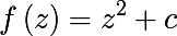
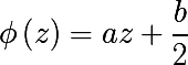
There is also the concept of a unitary ( a = 1 ) centered ( b = 0 ) form of a quadratic polynomial.



Introduce the following mapping φ , and find its inverse mapping:





Consider the following expression



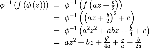
It is easy to see that the last expression resembles a quadratic polynomial in the general form of p (z) , let's find a c such that the resulting expression is reduced to a quadratic polynomial of general form



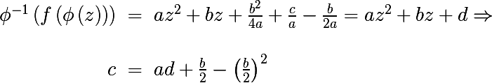
Thus, we have shown that with the above replacement c , a generalized polynomial can be written as

Behavior of a quadratic polynomial under the action of iterations

We turn to the third pebble base for understanding the Julia set. Consider the second iteration of the complex quadratic polynomial



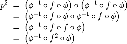
Not hard to show that



And just here we combine all three points, let's formulate a conclusion: in order to investigate the behavior of a quadratic polynomial under the action of iterations, it is enough to examine it in a unitary centered form, and not in general form . And this is really cool, because in general, we have as many as three coefficients, and in the unitary centered form only one.

Chaotic and normal behavior

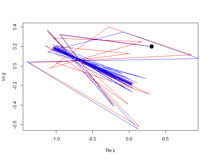
Soon it will be possible to give a definition of Julia's set. We will consider more intuitive definitions than strictly mathematical ones. But first, consider the concept of sustainability. The solution of a certain differential equation is called stable if the behavior of the solution with conditions close to the initial conditions is not much different from the behavior of the original solution. It is not difficult to guess that all the salt in the phrase is not much different . In general, various types of stability are distinguished, for example, Lyapunov stability is involved in the definition of the Julia set (this clearer definition follows from the Montel theorem on a compact family of functions ), but we will not even go into the essence of the differences in stability, here the main thing is to understand the idea. Let's try to illustrate it. To begin with, let's take a look at the intuitive perception of stability, here the blue and yellow trajectories of points with a small change behave almost the same, while for the red trajectory, a small change leads in a completely different direction.



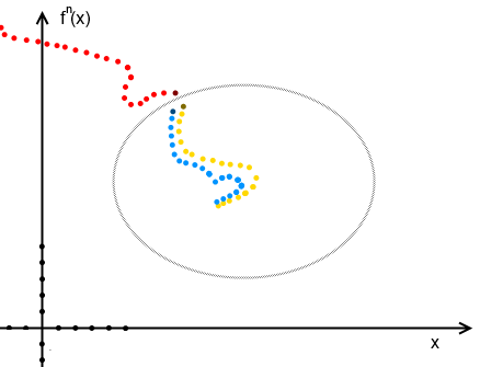
Let's consider the following polynomial f (z) = z ² - 1 + 0.213i , and construct a trajectory for 100 iterations with z ₀ = 0.3 + 0.2 i and z ₀ = 0.31 + 0.2 i



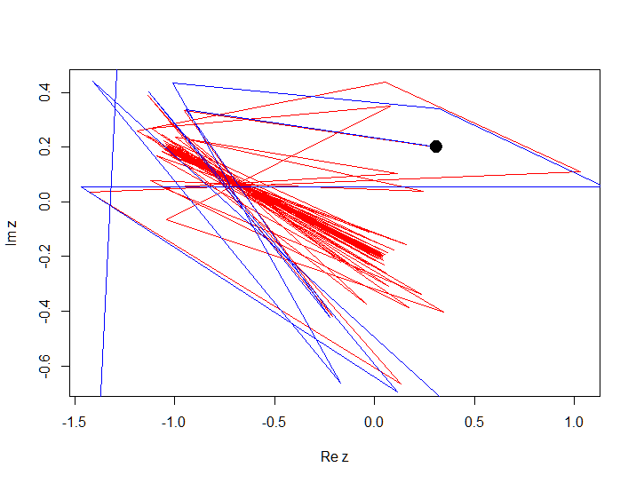
In this example, you see that a small change in the initial condition resulted in a divergence of the trajectories, we call this behavior chaotic in a certain neighborhood of the initial point, i.e. behavior strongly depends on small changes in the initial conditions. While the behavior under which stability is maintained, i.e. small changes in the initial conditions do not strongly affect the behavior in general, we will call normal, as in the following example. Consider the following polynomial f (z) = z ² - 1 + 0.2i (just slightly changed the constant c ), and construct a trajectory for 100 iterations at z ₀ = 0.3 + 0.2i and z ₀ = 0.31 + 0.2i

Fatu, Julia and Mandelbrot sets

• The Fatu set of the polynomial f (z) = z ² + c is a subset of the set of complex numbers, for each point of which, the behavior of the function under the action of iterations is normal , i.e. the trajectory of points generated by iterations does not change much with changing initial conditions in some small neighborhood of the initial point. Denoted by f (f) .
• The Julia set of the polynomial f (z) = z ² + c, respectively, is a subset of the set of complex numbers, for each point of which, the behavior of the function under the action of iterations is chaotic ; small changes in the initial conditions in some small neighborhood of the initial point, significantly affect the trajectory. Denoted by j (f)
• The Mandelbrot set is such a set of parameters c of the polynomial f (z) = z ² + c for which the Julia set is connected .

Attractor Pool

So we learned the meaning of the Julia set, we can proceed to the algorithm for constructing such a set. But for this, it is necessary first to introduce some other definitions.

• An attractor is a set of states of a dynamic system, in the direction of which the system develops over time. In our case, we can understand by the attractor a subset of fixed points to which sequences of iterations of the function converge, regardless of the initial conditions.
• The basin of an attractor of a point z of a function f is a subset of points from a neighborhood of z (denoted as A (z) ), such that any trajectory started at one of these points converges to a point z
• The pool of an attractor to infinity A (∞) is the set of those points z for which the trajectories go to infinity, that is, in other words, they do not converge to a fixed point, nor do they oscillate between two or more periodic points (a fixed point is a periodic point with a period equal to one).

Consider A (∞) in the context of our reasoning for some polynomial f (z) = z ² + c



It turns out that the following theorem exists. The set A (∞) (in the context described above) is open , connected and unbounded . It is fully contained in the set of veils . Julia set coincides with the boundary A (∞) , which is a closed and bounded subset of all complex numbers.

Constructing the Julia Set

I remind you that we will write an algorithm for constructing the Julia set of quadratic dynamics , and not any function. So, we learned that the Julia set coincides with the boundary A (∞) , which is a closed and bounded subset of all complex numbers, i.e. Julia's set is also closed and bounded. Let us denote as follows the subset of complex numbers that is generated by iterations of the function f and remains bounded. We call such a set a filled Julia set :



And the last theorem that we need sounds like this:

• Let some quadratic polynomial of the form f (z) = z ² + c be given
• denote
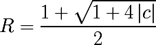
• then for some point and n> 0 the following condition is satisfied
• 
• those. if the module of the nth iteration is greater than R , then the iterations of the function f diverge, this is equivalent to the fact that the point z ₀ enters the pool of the attractor to infinity, which means that z _{0 is} not a point of the filled Julia set

In addition to the algorithm itself, it can be concluded from this theorem that the entire Julia set is inside a ball of radius R with center at the origin.

PS: approximately here lovers of design and golden sections, mystics and occult, will notice that with f (z) = z ² + 1 , the threshold R is equal to the golden section o_0

Algorithm

1. Choose c to set the polynomial f (z) = z ² + s
2. Calculate R for a given polynomial f (z) = z ² + s
3. We select the maxIter parameter to designate the maximum iteration, obviously the higher it is, the better the accuracy, the slower the algorithm
4. We generate an array of colors, the total maxIter pieces, say from less bright to brighter, we denote by color, how far away is the point from the Julia set
5. For each point, we calculate whether it is part of the filled Julia set or not, as well as the iteration number at which the threshold was exceeded
6. if | z | > R then use the first color, then use the light on which iteration number the threshold was exceeded

results

Here are a few of the 5k to 5k pictures made using this feature.

• f (z) = z ² - 0.8 + 0.156i
• f (z) = z ² + 0.285 + 0.01i
• f (z) = z ² - 0.0085 + 0.71i

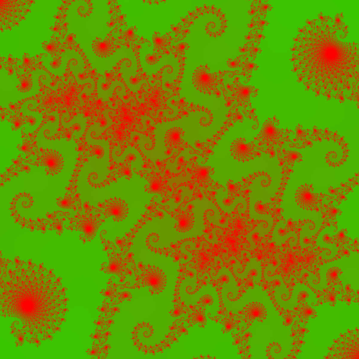
And now let's look at the Julia set for the polynomial f (z) = z ² - 0.74543 + 0.11301i , the whole set is contained in the ball of radius 1.50197192317588 .













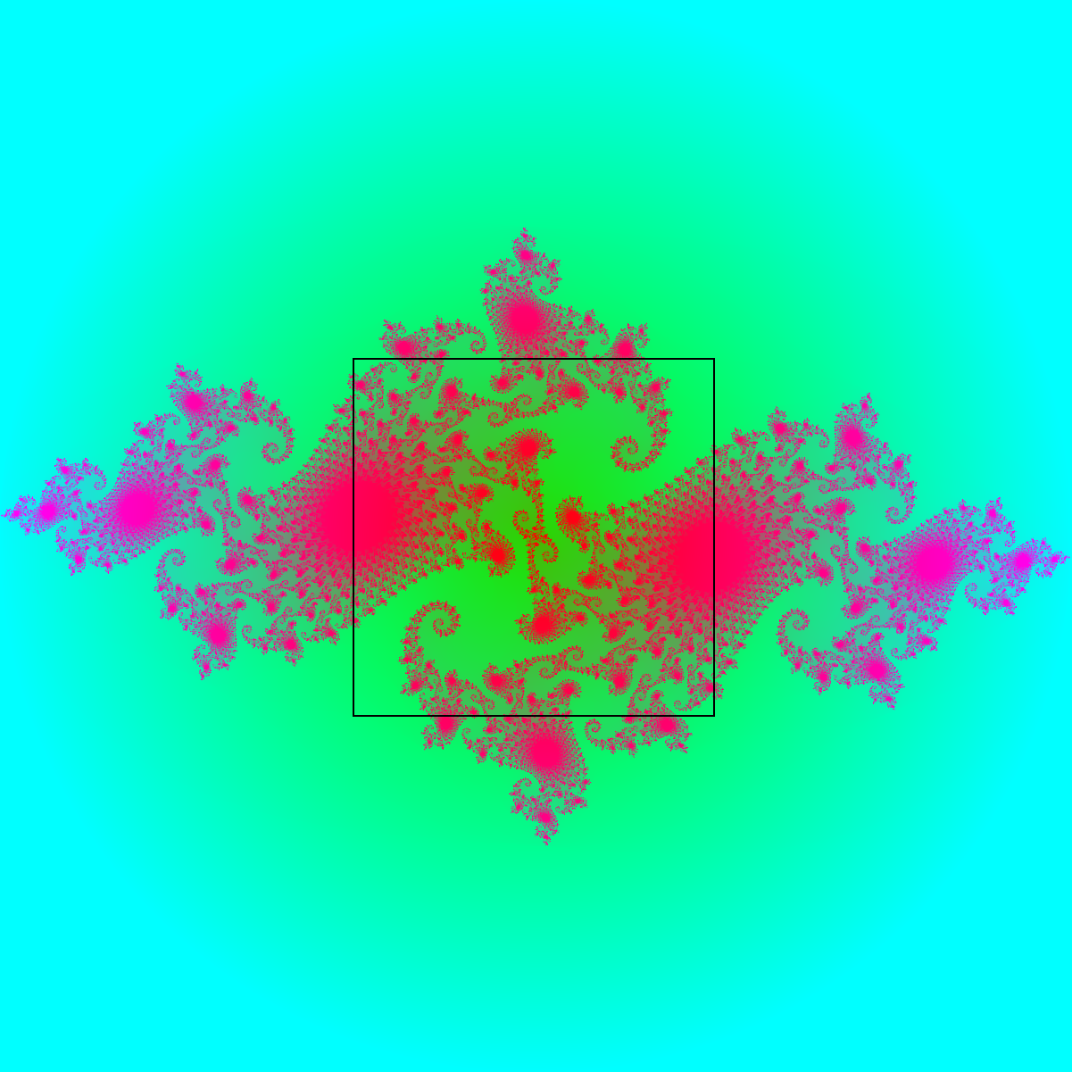
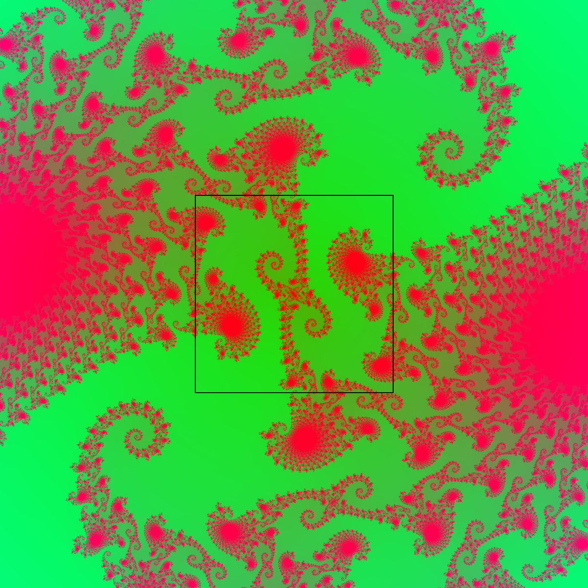
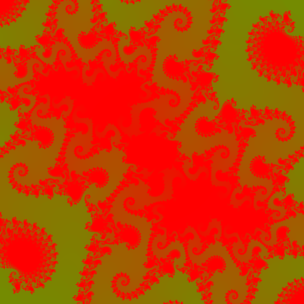
Approximately on this picture it seems that the limit of accuracy has been reached, and all the red elements belong to the set of Julia. But it was not there, we increase the maxIter parameter, and we get an even more accurate approximation. In general, you can continue indefinitely. No kidding -)