Inventing JPEG
You correctly understood from the title that this is not an ordinary description of the JPEG algorithm (I described the file format in detail in the article "JPEG decoding for dummies" ). First of all, the chosen method of presenting the material assumes that we know nothing not only about JPEG, but also about the Fourier transform, and Huffman coding. And in general, there is little to remember from the lectures. Just took the picture and began to think how it can be compressed. Therefore, I tried to expressly express only the essence, but at which the reader will have a sufficiently deep and, most importantly, an intuitive understanding of the algorithm. Formulas and mathematical calculations - at the very minimum, only those that are important for understanding what is happening.
Knowledge of the JPEG algorithm is very useful not only for image compression. It uses the theory of digital signal processing, mathematical analysis, linear algebra, information theory, in particular, Fourier transform, lossless coding, etc. Therefore, this knowledge can be useful anywhere.
If there is a desire, then I propose to go through the same stages independently in parallel with the article. Check how the above reasoning is suitable for different images, try to make your own modifications to the algorithm. It is very interesting. As a tool, I can recommend a wonderful bundle of Python + NumPy + Matplotlib + PIL (Pillow). Almost all of my work (including graphics and animation) was done using them.
')
Attention, traffic! Many illustrations, graphs and animations (~ 10Mb). Ironically, the article about JPEG only 2 images with this format of fifty.
Whatever the algorithm for compressing information, its principle will always be the same - finding and describing patterns. The more patterns, the more redundancy, the less information. Archivers and coders are usually “sharpened” for a specific type of information, and they know where to find them. In some cases, the pattern is visible immediately, for example, a picture of a blue sky. Each row of its digital representation can be fairly accurately described as straight.
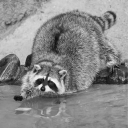
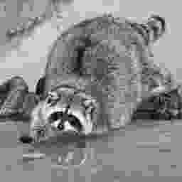
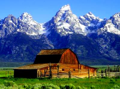
We will train on
Vector presentation
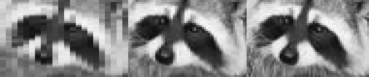
First, let's check how dependent two neighboring pixels are. It is logical to assume that most likely they will be very similar. Check it out for all image pairs. Mark them on the coordinate plane with dots so that the point value along the X axis is the value of the first pixel, along the Y axis it is the second one. For our image of 256 by 256 we get 256 * 256/2 points:

It is predicted that most of the points are on or near the straight line y = x (and there are even more of them than can be seen in the figure, since they repeatedly overlap each other, and, moreover, they are translucent). And if so, it would be easier to work by turning them through 45 °. To do this, express them in a different coordinate system.
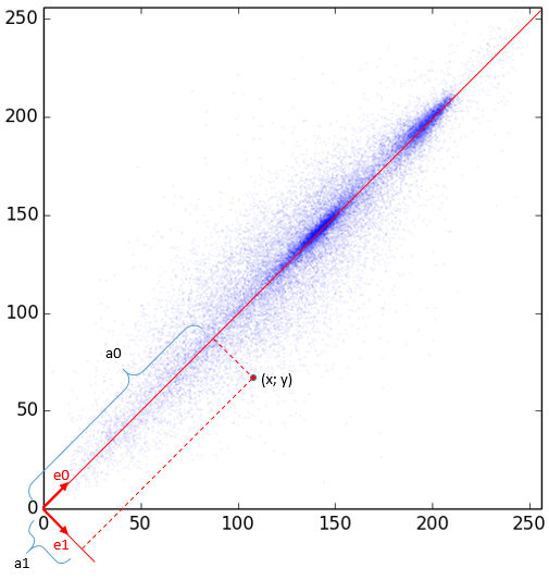
The base vectors of the new system are obviously:
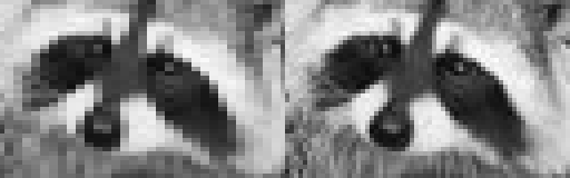
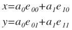
 . They are forced to divide by the root of two to get an orthonormal system (the lengths of the basis vectors are equal to unity). Here it is shown that some point p = (x, y) in the new system will be represented as a point (a 0 , a 1 ). Knowing the new coefficients, we can easily get the old reverse turn. Obviously, the first (new) coordinate is the average, and the second is the difference between x and y (but divided by the root of 2). Imagine that you are asked to leave only one of the values: either a 0 or a 1 (i.e., equate another to zero). It is better to choose a 0 , since the value of a 1 is likely to be around zero. Here's what happens if we restore the image only at a 0 :
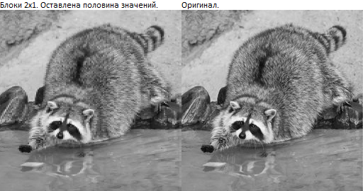
4 times magnification:
Such compression is not very impressive, to be honest. It is better to similarly divide the image into triples of pixels and represent them in three-dimensional space.


This is the same graph, but from different points of view. The red lines are the axes that have been asking for themselves. They correspond to the vector:
 . I remind you that you have to divide into some constants so that the lengths of the vectors become equal to one. Thus, expanding on such a basis, we get 3 values a 0 , a 1 , a 2 , and a 0 is more important than a 1 , and a 1 is more important than a 2 . If we drop a 2 , then the graph “flattens out” in the direction of the vector e 2 . This and so is not quite thick three-dimensional sheet will be flat. It will lose not so much, but we will get rid of a third of the values. Compare the images reconstructed in triples: (a 0 , 0, 0), (a 1 , a 2 , 0) and (a 0 , a 1 , a 2 ). In the last version, we did not throw anything away, so we get the original.
4 times magnification:
The second picture is already good. The sharp areas smoothed out a bit, but on the whole the picture was preserved very well. And now, in the same way, we divide into fours and visually define the basis in four-dimensional space ... Oh, yes. But one can guess what one of the basis vectors will be: (1,1,1,1) / 2. Therefore, you can look at the projection of the four-dimensional space on the space perpendicular to the vector (1,1,1,1), in order to identify others. But this is not the best way.
Our goal is to learn how to transform (x 0 , x 1 , ..., x n-1 ) to (a 0 , a 1 , ..., a n-1 ) so that each value of a i is less important than previous If we can do this, then perhaps the last sequence values can be thrown away altogether. The above experiments hint that you can. But one cannot do without a mathematical apparatus.
So, you need to convert the points to a new basis. But first you need to find a suitable basis. Let us return to the first experiment of splitting into pairs. We will consider it generically. We defined the basis vectors:

Express through them the vector p :

or in coordinates:
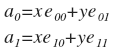
To find a 0 and a 1, you need to project p onto e 0 and e 1, respectively. And for this you need to find the scalar product

similarly:

In coordinates:
It is often more convenient to perform the transformation in matrix form.
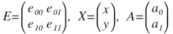
Then A = EX and X = E T A. This is a beautiful and convenient form. The matrix E is called the transformation matrix and is orthogonal; we will still meet with it.
Transition from vectors to functions.
It is convenient to work with vectors of small dimensions. However, we want to find patterns in larger blocks, so instead of N-dimensional vectors it is more convenient to operate with sequences that represent the image. I will call such sequences discrete functions, since the following reasoning applies to continuous functions.
Returning to our example, we represent such a function f (i), which is defined only at two points: f (0) = x and f (1) = y. Similarly, we define the basis functions e 0 (i) and e 1 (i) on the basis of the bases e 0 and e 1 . We get:
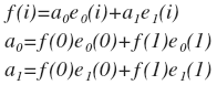
This is a very important conclusion. Now in the phrase “decomposition of a vector in orthonormal vectors” we can replace the word “vector” by “function” and get a completely correct expression “decomposition of a function in orthonormal functions”. It does not matter that we received such a short function, since the same reasoning works for the N-dimensional vector, which can be represented as a discrete function with N values. And working with functions is clearer than with N-dimensional vectors. It is possible, and vice versa, to present such a function as a vector. Moreover, an ordinary continuous function can be represented by an infinite-dimensional vector, though not in a Euclidean, but a Hilbert space. But we will not go there, we will be interested only in discrete functions.
And our task of finding a basis turns into the problem of finding a suitable system of orthonormal functions. In the following reasoning, it is assumed that we have somehow defined a set of basis functions by which we will decompose.
Suppose we have a certain function (represented by, for example, values) that we want to represent as a sum of others. You can represent this process in vector form. To decompose a function, you need to “project” it into basic functions in turn. In the vector sense, the calculation of the projection gives the minimum approximation of the original vector to another in distance. Remembering that the distance is calculated using the Pythagorean theorem, then a similar representation in the form of functions gives the best rms approximation of the function to another. Thus, each coefficient (k) determines the "proximity" of the function. More formally, k * e (x) is the best rms approximation to f (x) among l * e (x).
The following example shows the process of approximating a function using only two points. On the right is a vector representation.

With reference to our pairing experiment, we can say that these two points (0 and 1 on the abscissa) are a pair of neighboring pixels (x, y).
The same, but with animation:
If we take 3 points, then we need to consider three-dimensional vectors, but the approximation will be more accurate. And for a discrete function with N values, we need to consider N-dimensional vectors.
Having a set of derived coefficients, one can easily obtain the original function by summing the basis functions taken with the corresponding coefficients. Analysis of these coefficients can provide a lot of useful information (depending on the basis). A special case of these considerations is the principle of expansion in a Fourier series. After all, our reasoning applies to any basis, and when decomposing into a Fourier series, it is taken quite concretely.
Discrete Fourier Transforms (DFT)
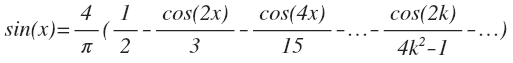
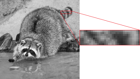
In the previous section, we concluded that it would be nice to decompose a function into components. In the early 19th century, Fourier also thought about this. True, he did not have a picture with a raccoon, so he had to investigate the distribution of heat along a metal ring. Then he found out that it is very convenient to express the temperature (and its change) at each point of the ring as the sum of sinusoids with different periods. “Fourier has established (I recommend to read , interestingly) that the second harmonic is damped 4 times faster than the first, and the harmonics of higher orders are damped with even greater speed.”
In general, it soon turned out that the periodic functions are remarkably decomposed into the sum of sinusoids. And since there are many objects and processes in nature that are described by periodic functions, a powerful tool for their analysis has appeared.
Perhaps one of the most illustrative periodic processes is sound.

- The 1st graph is a pure tone with a frequency of 2500 hertz.
- 2nd - white noise. That is, noise with evenly distributed frequencies throughout the range.
- 3rd is the sum of the first two.
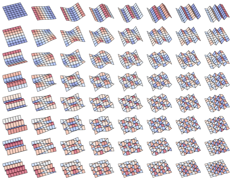
Why not try to take a sine wave as a basis? In fact, we have actually done it. Recall our decomposition into 3 basis vectors and plot them on the graph:

Yes, yes, I know, it looks like a fit, but with three vectors it's hard to expect more. But now it is clear how to get, for example, 8 basic vectors:
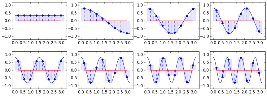
A not very complicated test shows that these vectors are pairwise perpendicular, that is, orthogonal. This means they can be used as a basis. Transformation over such a basis is widely known, and is called discrete cosine transform (DCT). I think from the graphs below it is clear how the DCT-conversion formula is obtained:

This is all the same formula: A = EX with a substituted basis. The basis vectors of the indicated DCT (they are the same row vectors of the matrix E) are orthogonal, but not orthonormal. This should be remembered during the inverse transformation (I will not dwell on this, but for whom it is interesting, the inverse DCT contains the term 0.5 * a 0 , since the zero basis vector is larger than the others).
The following example shows the process of approximating subtotals to baseline values. At each iteration, the regular basis is multiplied by the next coefficient and added to the subtotal (that is, just like in the earlier experiments on the raccoon, one third of the values, two thirds).
But, nevertheless, despite some arguments about the advisability of choosing such a basis, there are no real arguments yet. Indeed, unlike sound, the expediency of decomposing an image into periodic functions is much less obvious. However, the image may indeed be too unpredictable even in a small area. Therefore, the picture is divided into fairly small pieces, but not quite tiny, so that the decomposition makes sense. In JPEG, the image is “sliced” into 8x8 squares. Within the limits of such a slice, photographs are usually very uniform: a background plus small fluctuations. Such areas are smartly approaching with sinusoids.
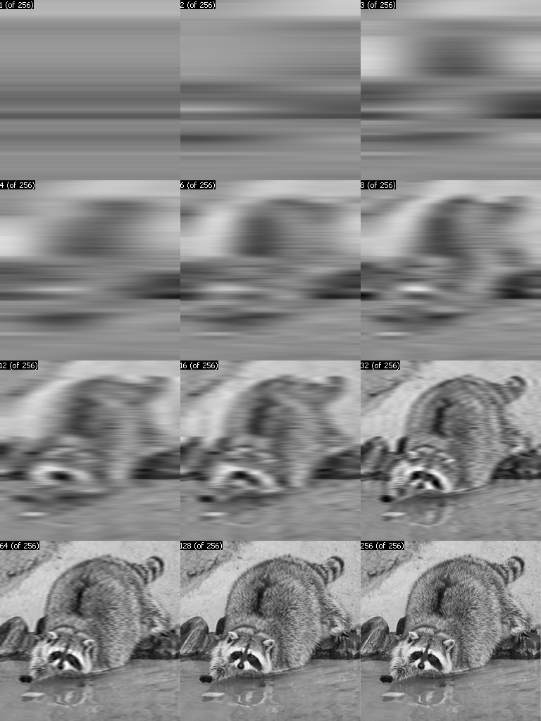
Well, let's say this fact is more or less intuitive. But there is a bad feeling about sharp color transitions, because slowly changing functions will not save us. It is necessary to add different high-frequency functions that cope with their work, but appear sideways on a uniform background. Take an image of 256x256 with two contrast areas:

We decompose each row with DCT, thus obtaining 256 coefficients per row.
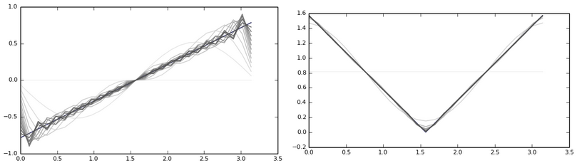
Then we leave only the first n coefficients, and the rest equate to zero, and, therefore, the image will be represented as a sum of only the first harmonics:

The number in the picture is the number of coefficients left. In the first image, only the mean value remains. The second has already added one low-frequency sine wave, and so on. By the way, pay attention to the border - despite all the best approximation, 2 bars are clearly visible near the diagonal, one is lighter, the other is darker. Part of the last image enlarged 4 times:

And generally, if far from the border we see the initial uniform background, then when approaching it, the amplitude begins to grow, finally reaches its minimum value, and then sharply becomes maximum. This phenomenon is known as the Gibbs effect.
The height of these humps, appearing near the discontinuities of the function, does not decrease with an increase in the number of the sum of the functions. In a discrete transformation, it disappears only when almost all coefficients are saved. More precisely, it becomes invisible.
The following example is completely analogous to the above decomposition of triangles, but already on a real raccoon:
When studying DCT, one may get the false impression that only the first few (low-frequency) coefficients are always enough. This is true for many pieces of photos, those whose values do not change dramatically. However, on the border of contrasting areas, the values will briskly “ride” and even the last coefficients will be great. Therefore, when you hear about the DCT energy conservation property, make a correction that it applies to many types of signals encountered, but not to all. For example, think about how a discrete function will look, the decomposition coefficients of which are zero, except for the last. Hint: Imagine decomposition in vector form.
Despite the shortcomings, the chosen basis is one of the best in real photographs. A little later we will see a small comparison with others.
DCT vs everything else
When I studied the issue of orthogonal transformations, then, frankly, I was not very convinced by the arguments that everything around was the sum of harmonic oscillations, therefore, the pictures should also be laid out on sinusoids. Or maybe some step functions would be better? Therefore, I was looking for research results on the optimality of DCT on real images. The fact that “It is DCT that is most often found in practical applications due to the property of“ energy compacting ”is written everywhere. This property means that the maximum amount of information is contained in the first coefficients. And why? It is not difficult to conduct a study: we arm ourselves with a bunch of different pictures, different known bases, and begin to consider the standard deviation from the real image for a different number of coefficients. Found a small study in the article (images used here ) by this method. It contains graphs of the dependence of the stored energy on the number of first expansion coefficients over different bases. If you looked at the charts, you made sure that the DCT is consistently honored ... um ... 3rd place. How so? What is KLT conversion? I praised the DCT, and here ...
KLT
All transformations, except KLT, are transformations with a constant basis. And in KLT (the Karhunen-Loeve transform) the most optimal basis for several vectors is calculated. It is calculated in such a way that the first coefficients give the smallest root-mean-square error for the total for all vectors. We carried out similar work earlier manually, visually defining the basis. At first it seems like a sensible idea. We could, for example, break an image into small sections and calculate a basis for each one. But not only is there a concern of storing this basis, so also the operation of calculating it is rather laborious. But DCT loses only a little, and besides DCT has fast conversion algorithms.
Dft
DFT (Discrete Fourier Transform) is a discrete Fourier transform. Under this name, not only a specific transformation is sometimes mentioned, but also the entire class of discrete transformations (DCT, DST ...). Let's look at the DFT formula:
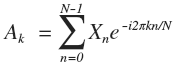
As you might guess, this is an orthogonal transformation with some kind of complex basis. Since such a complex form occurs a little more often than always, it makes sense to study its conclusion.
It may appear that any pure harmonic signal (with an integer frequency) during DCT decomposition will produce only one non-zero coefficient corresponding to this harmonic. This is not the case, because besides the frequency, the phase of this signal is important. For example, the decomposition of a sine in cosines (in a similar way and in discrete decomposition) would be:
So much for pure harmonics. She spawned a bunch of others. The animation shows the DCT coefficients of the sine wave in different phases.
If it seemed to you that the columns rotate around an axis, then you did not think.
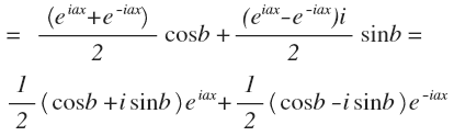
So now we will expand the function on the sum of the sinusoids not just of different frequencies, but also shifted in some phase. It will be more convenient to consider the phase shift using the example of cosine:

A simple trigonometric identity gives an important result: the phase shift is replaced by the sum of sine and cosine, taken with the coefficients cos (b) and sin (b). So, you can decompose the functions on the sum of sines and cosines (without any phases). This is a common trigonometric form. However, complex is more often used. To obtain it you need to use the Euler formula.. Just substitute the derived formulas for sine and cosine, we get:
Now a small substitution. Upper underscore is the conjugate number.

We obtain the final equality:

c is the complex coefficient, the real part of which is equal to the cosine coefficient, and the imaginary part - to the sine. And the set of points (cos (b), sin (b)) is a circle. In such a record, each harmonic is included in the decomposition with both positive and negative frequencies. Therefore, summation or integration from minus to plus infinity usually occurs in various formulas of Fourier analysis. It is often more convenient to perform calculations in such a complex form.
The transformation decomposes the signal into harmonics with frequencies from one to N oscillations in the signal region. But the sampling rate is N on the signal area. And according to the Kotelnikov theorem (aka the Nyquist – Shannon theorem), the sampling frequency should be at least twice the signal frequency. If this is not the case, then the effect of the appearance of a signal with a false frequency is obtained:
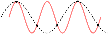
Dotted lines show an incorrectly restored signal. With this phenomenon you often come across in life. For example, a fun movement of the wheels of a car in the video, or a moire effect.
This leads to the fact that the second half of the N complex amplitudes seem to consist of other frequencies. These false harmonics of the second half are a mirror image of the first and do not carry additional information. Thus, we have N / 2 cosines and N / 2 sines (forming an orthogonal basis).
Well, there is a basis. Its components are harmonics with an integer number of oscillations on the signal region, and therefore, the extreme values of the harmonics are equal. More precisely, they are almost equal, since the latter value is taken not entirely from the edge. Moreover, each harmonic is almost mirror-symmetrical about its center. All these phenomena are especially strong at low frequencies, which are important to us in coding. This is also bad because the block borders will be visible on the compressed image. I illustrate the DFT-basis with N = 8. The first 2 rows are cosine components, the last ones are sinus:
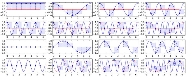
Pay attention to the appearance of duplicate components with increasing frequency.
You can think mentally how a signal could be decomposed, the values of which gradually decrease from the maximum value at the beginning to the minimum at the end. A more or less adequate approximation could only make the harmonics closer to the end, which is not very good for us. The figure on the left is the asymmetric signal approximation. Right - symmetrical:
From the first case is extremely bad.
So it can be done like in DCT - to reduce the frequency by 2 or another number of times so that the number of some oscillations is fractional and the boundaries are in different phases? Then the components will be non-orthogonal. And nothing can be done about it.
DST
What if instead of cosines in DCT use sines? We get the Discrete Sine Transform (DST). But for our task, they are all uninteresting, since both the whole and the halves of the sinus periods are close to zero at the boundaries. That is, we get about the same inappropriate decomposition, as in the DFT.
Returning to DCT
How is he doing at the borders? Good. There are antiphases and no zeros.
All the rest
Non-Fourier transform. I will not describe.
WHT - the matrix consists only of step components with values of -1 and 1.
Haar is partly orthogonal wavelet transform.
They are inferior to DCT, but easier to compute.
So, the thought came to you to invent your own transformation. Remember this:
- The basis must be orthogonal.
- With a fixed basis, you cannot outperform KLT in compression quality. Meanwhile, on real photos DCT is almost as good.
- For example, DFT and DST need to remember about the border.
- And remember that DCT has another good advantage - near the boundaries of the components that make up their derivatives are zero, which means that the transition between adjacent blocks will be fairly smooth.
- Fourier transforms have fast algorithms with complexity O (N * logN), as opposed to head-on: O (N 2 ).
It won't be easy, right? However, for some types of images you can choose a better basis than the DCT.
This section turned out to be similar to a discrete cosine transform advertisement. But it is really cool!
2D transformations
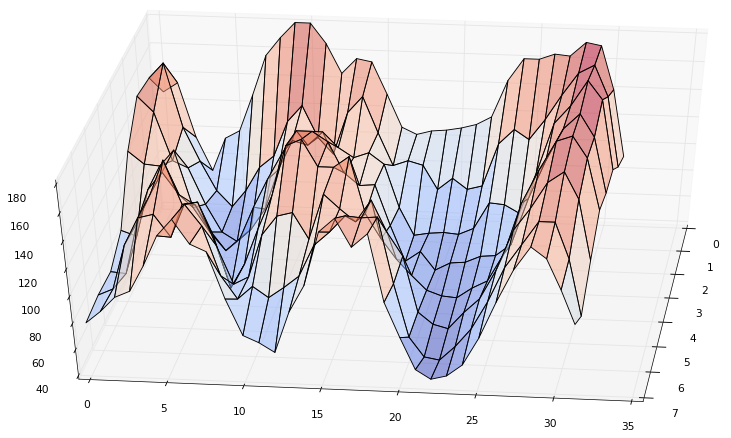
Now we will try to conduct such an experiment. Take, for example, a piece of the image.
His 3D graph:
Go through DCT (N = 32) for each line:

Now I want you to run your eyes over each column of the obtained coefficients, i.e. from top to bottom. Recall that our goal is to leave as few values as possible, removing the minor ones. Surely you guessed that the values of each column of the obtained coefficients can be decomposed in the same way as the values of the original image. No one restricts us in choosing an orthogonal transformation matrix, but we will do it again using DCT (N = 8):

The coefficient (0,0) turned out to be too large, so on the graph it is reduced by 4 times.
So what happened?
The upper left corner is the most significant expansion coefficients of the most significant coefficients.
The lower left corner is the most insignificant coefficients of the expansion of the most significant coefficients.
The upper right corner is the most significant expansion coefficients of the most insignificant coefficients.
The lower right corner is the most insignificant expansion coefficients of the most insignificant coefficients.
It is clear that the significance of the coefficients decreases if you move diagonally from the upper left to the lower right. And which is more important: (0, 7) or (7, 0)? What do they even mean?
First line by line: A 0 = (EX T )T = XE T (transposed, since the formula A = EX columns) then the columns: A = EA 0 = EXE T . If we carefully calculate, we get the formula:
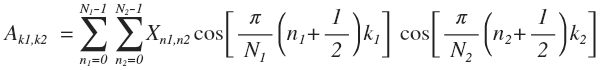
Thus, if the vector is decomposed into sinusoids, then the matrix on functions of the form cos (ax) * cos (by). Each block of 8x8 in JPEG is represented as a sum of 64 functions of the form:
In Wikipedia and other sources, such functions are presented in a more convenient form:
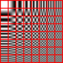
Therefore, the coefficients (0, 7) or (7, 0) are equally useful.
However, in fact, this is the usual one-dimensional decomposition on 64 64-dimensional basis. All of the above applies not only to DCT, but also to any orthogonal decomposition. Acting by analogy, in the general case we obtain an N-dimensional orthogonal transform.
And here is a 2-dimensional transformation of a raccoon (DCT 256x256). Again with zeroed values. Numbers - the number of non-zero coefficients of all (the most significant values were left, which are in a triangular area in the upper left corner).

Remember that the coefficient (0, 0) is called DC, the other 63 is AC.
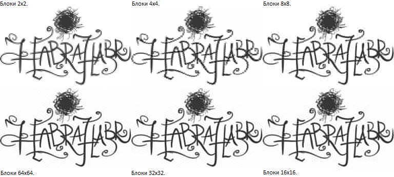
Select block size
A comrade asks : why in JPEG is the 8x8 split used. From the spiteful answer:
It has been the case for the DCT. If you take 64x64 blocks, you will have toThey say that DCT works well only on periodic functions, and if you take a large size, you will most likely get a giant leap at the block boundaries and you will need a lot of high-frequency components to cover it. This is not true! Such an explanation is very similar to the DFT, but not to the DCT, as it perfectly covers such jumps by the very first components.
On the same page is the answer from the MPEG FAQ, with the main arguments against the big blocks:
- Little profit when split into large blocks.
- Increase computational complexity.
- , .
I suggest to investigate it yourself. Let's start with the first .
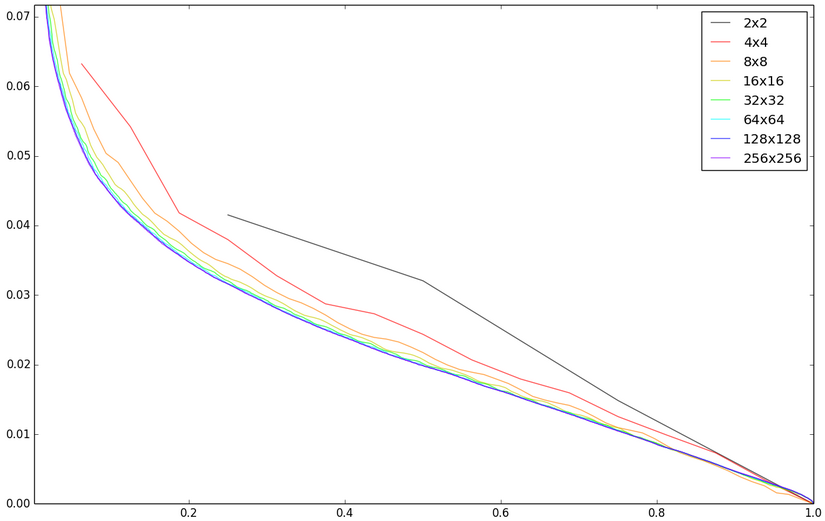
The horizontal axis is the fraction of the first non-zero coefficients. Vertical - the standard deviation of pixels from the original. The maximum possible deviation is taken per unit. Of course, one picture is clearly not enough for the verdict. Besides, I'm not acting quite correctly, just zeroing. In real JPEG, depending on the quantization matrix, only small values of high-frequency components are zeroed. Therefore, the following experiments and conclusions are intended to superficially identify principles and patterns.
You can compare the division into different blocks with the left 25 percent of the coefficients (from left to right, then from right to left):

Large blocks are not shown, as they are visually almost indistinguishable from 32x32. Now let's look at the absolute difference with the original image (amplified 2 times, otherwise nothing really can be seen):
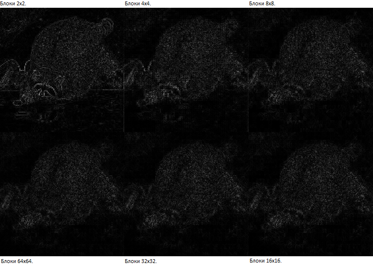
8x8 gives a better result than 4x4. A further increase in size does not give a well-marked advantage. Although I would seriously think about 16x16, instead of 8x8: an increase of 33% in complexity (of the complexity in the next paragraph) gives a small but still visible improvement with the same number of coefficients. However, the choice of 8x8 looks quite reasonable and, perhaps, is the golden mean. JPEG was published in 1991. I think that such compression was very difficult for processors of that time.
Secondargument. It must be remembered that increasing the block size will require more calculations. Let's evaluate how much. The complexity of the transformation in the forehead, as we already know how to: O (N 2 ), since each coefficient consists of N terms. But in practice, an efficient fast Fourier transform algorithm (FFT, Fast Fourier Transform, FFT) is used. His description is beyond the scope of the article. Its complexity: O (N * logN). For two-dimensional decomposition, you need to use it twice N times. Thus, the complexity of the 2D DCT - O (N 2 logN). Now let's compare the complexity of computing an image with one block and several small ones:
- In one block (kN) x (kN): O ((kN) 2 log (kN)) = O (k 2 N 2 log (kN))
- k * k in N * N: O blocks (k 2 N 2 logN)
This means that, for example, computing when split into 64x64 is two times more complicated than it is into 8x8.
The third argument. If we have a sharp border of flowers on the image, then this will affect the whole block. Perhaps this block will be better enough small, because in many neighboring blocks, such a border is likely to be gone. However, far from the boundaries, the attenuation occurs fairly quickly. In addition, the border itself will look better. Let's check with an example with a large number of contrasting transitions, again, with only a quarter of the coefficients:
Although the distortions of the 16x16 blocks extend further than that of 8x8, but the inscription is smoother. Therefore, I was convinced only the first two arguments. But something more like 16x16 divisions.
Quantization
At this stage, we have a bunch of 8x8 matrices with cosine transform coefficients. It's time to get rid of unimportant coefficients. There is a more elegant solution than simply resetting the last coefficients, as we did above. We are not satisfied with this method, since non-zero values are stored with excessive accuracy, and among those who are not lucky, they could be quite important. Output - you need to use a quantization matrix. Losses occur at this stage. Each Fourier coefficient is divided by the corresponding number in the quantization matrix. Consider an example. Take the first block from our raccoon and produce quantization. The JPEG specification provides the standard matrix:
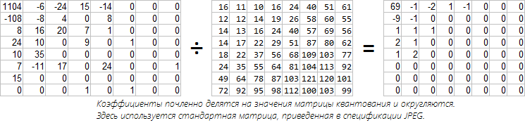
The standard matrix corresponds to 50% quality in FastStone and IrfanView. Such a table was chosen in terms of the balance of quality and degree of compression. I think that the value for the DC coefficient is greater than the neighboring ones due to the fact that DCT is not normalized and the first value is obtained more than it should. High-frequency coefficients are rougher because of their lesser importance. I think that now such matrices are rarely used, since the deterioration is well marked. Nobody forbids to use your table (with values from 1 to 255)
When decoding, the inverse process occurs - the quantized coefficients are multiplied by the term of time by the values of the quantization matrix. But since we are rounding the values, we will not be able to accurately restore the original Fourier coefficients. The greater the quantization number, the greater the error. Thus, the restored coefficient is only the nearest multiple.
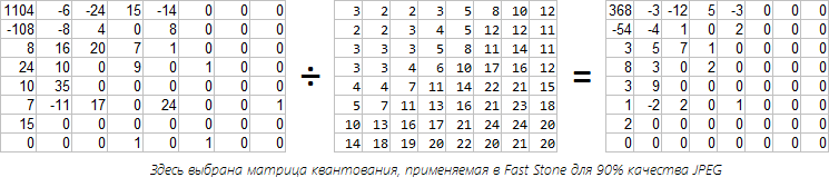
Another example:
And for dessert, consider the quality of 5% (when coding in Fast Stone).
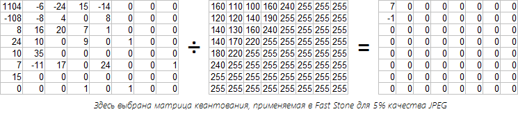
When restoring this block, we get only the averaged value plus the vertical gradient (due to the preserved value of -1). But for him only two values are stored: 7 and -1. With other blocks, the situation is no better, here is the restored picture:
By the way, about 100% quality. As you might guess, in this case the quantization matrix consists entirely of units, that is, no quantization occurs. However, due to the rounding of the coefficients to the whole, we cannot exactly restore the original image. For example, a raccoon kept 96% of pixels exactly, and 4% differed by 1/256. Of course, such “distortions” cannot be seen visually.
And here you can see the quantization matrix of various cameras.
Coding
Before proceeding further, we need to understand with simpler examples how to compress the values obtained.
Example 0 (for warm-up)
Imagine such a situation that your friend has forgotten a list with a list in your house and now asks to dictate it by telephone (there are no other means of communication).
List:
- d9rg3
- wfr43gt
- wfr43gt
- d9rg3
- d9rg3
- d9rg3
- wfr43gt
- d9rg3
How would you make your task easier? You have no particular desire to dictate all these words. But there are only two of them and they are repeated. Therefore, you just somehow dictate the first two words and agree that further “d9rg3” will be called the first word, and “wfr43gt” - the second. Then it will be enough to dictate: 1, 2, 2, 1, 1, 1, 2, 1.
We will denote such words as A, B, C ..., and call them symbols. And under the symbol can hide anything: a letter of the alphabet, a word or a hippopotamus in a zoo. The main thing is that the same symbols correspond to the same concepts, but different to different. Since our task is efficient coding (compression), we will work with bits, since these are the smallest units of information representation. Therefore, we write the list as ABBAAABA. Instead of “first word” and “second word”, you can use bits 0 and 1. Then ABBAAABA is encoded as 01100010 (8 bits = 1 byte).
Example 1
Encode ABC.
3 different symbols (A, B, C) can not be compared with 2 possible values of bits (0 and 1). And if so, then you can use 2 bits per symbol. For example:
- A: 00
- B: 01
- C: 10
The sequence of bits associated with a symbol will be called a code. ABC will be encoded as: 000110.
Example 2
Encode AAAAAABC.
Using 2 bits per symbol A seems a bit wasteful. What if you try this:
- A: 0
- B: 1
- C: 00

Encoded sequence: 000000100.
Obviously, this option is not suitable, since it is not clear how to decode the first two bits of this sequence: as AA or as C? It is very wasteful to use any separator between the codes, we will think how to get around this obstacle in a different way. So, the failure occurred because the C code starts with the A code. But we are determined to encode A in one bit, even if B and C are two each. Proceeding from such a wish, A will give code 0. Then codes B and C cannot begin at 0. But they can by 1:
- A: 0
- B: 10
- C: 11

The sequence is encoded as: 0000001011. Try to mentally decode it. You can only do this in one way.
We have developed two coding requirements:
- The greater the weight of the character, the shorter its code should be. And vice versa.
- For unambiguous decoding, the character code cannot begin with the code of any other character.
Obviously, the order of characters is not important, we are only interested in the frequency of their occurrence. Therefore, with each symbol is assigned a number, called weight. The weight of a symbol can be both a relative value, reflecting the proportion of its occurrence, and absolute, equal to the number of symbols. The main thing is that the weights should be proportional to the occurrence of characters.
Example 3
Consider the general case for 4 characters with any weights.
- A: pa
- B: pb
- C: pc
- D: pd
Without loss of generality, we put pa ≥ pb ≥ pc ≥ pd. There are only two variant codes that are fundamentally different in length:

Which one is preferable? To do this, calculate the lengths of the encoded messages:
W1 = 2 * pa + 2 * pb + 2 * pc + 2 * pd
W2 = pa + 2 * pb + 3 * pc + 3 * pd
If W1 is less than W2 (W1-W2 <0), then it is better to use the first option:
W1-W2 = pa - (pc + pd) <0 => pa <pc + pd.
If C and D together occur more often than others, then their common vertex gets the shortest code of one bit. Otherwise, one bit goes to symbol A. Hence, the combination of characters behaves as an independent character and has a weight equal to the sum of the incoming characters.
In general, if p is the weight of a character represented by a fraction of its occurrence (from 0 to 1), then the best code length is s = -log 2 p.
Consider this in a simple case (it is easy to imagine it as a tree). So, you need to encode 2 s characters with equal weights (1/2 s ). Due to the equality of the weights, the length of the codes will be the same. Each character will require s bits. So, if the weight of the symbol is 1/2 s , then its length is s. If we replace the weight with p, then we get the length of the code
And one more observation - the two characters with the smallest weights always have the greatest, but equal lengths of codes. Moreover, their bits, except the last one, coincide. If this were not true, then at least one code could be shortened by 1 bit without violating the prefix. This means that the two characters with the smallest weights in the code tree have a common parent a level higher. You can see this in the example of C and D above.
Example 4
Let's try to solve the following example, according to the conclusions obtained in the previous example.
- All characters are sorted in descending order of weights.
- The last two characters are grouped together. This group is assigned a weight equal to the sum of the weights of these elements. This group participates in the algorithm along with symbols and other groups.
The steps are repeated until there is only one group left. In each group, one character (or subgroup) is assigned bit 0, and the other bit 1.
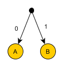
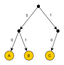
This algorithm is called Huffman coding.
The illustration shows an example with 5 characters (A: 8, B: 6, C: 5, D: 4, E: 3). On the right is the weight of the symbol (or group).

We code coefficients
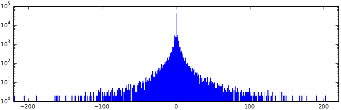
Come back. Now we have a lot of blocks with 64th coefficients in each, which need to somehow be saved. The simplest solution is to use a fixed number of bits per coefficient — obviously, unfortunate. Construct a histogram of all obtained values (i.e., the dependence of the number of coefficients on their value):

Pay attention - the logarithmic scale! Can you explain the reason for the accumulation of values greater than 200? These are DC coefficients. Since they are very different from the rest, it is not surprising that they are encoded separately. Here are just DC:
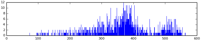
Notice that the shape of the graph resembles the shape of the graphs from the very early experiments of dividing into pairs and triples of pixels.
In general, the values of DC coefficients can vary from 0 to 2047 (more precisely, from -1024 to 1023, since 128 is subtracted from JPEG from all the original values, which corresponds to 1024 subtraction from DC) and distributed fairly evenly with small peaks. Therefore, Huffman coding is not very helpful. Imagine how big the coding tree will be! And during decoding you will have to look for values in it. It is very expensive. We think further.
DC coefficient - averaged value of 8x8 block. Imagine a gradient transition (albeit not perfect), which is often found in photographs. The DC values themselves will be different, but they will represent an arithmetic progression. Hence, their difference will be more or less constant. Construct a histogram of differences:

Now this is better, because the values are generally concentrated around zero (but the Huffman algorithm will again give too large a tree). Small values (in absolute value) are common, large rarely. And since small values take up little bits (if you remove leading zeros), one of the compression rules is well executed: assign short codes to symbols with large weights (and vice versa). We are still limited by the failure to comply with another rule: the impossibility of unambiguous decoding. In general, such a problem is solved in the following ways: confuse with the code separator, specify the length of the code, use prefix codes (you already know them - this is the case when no code starts with another). Let's go with the simple second variant, i.e. each coefficient (more precisely, the difference of the neighboring ones) will be written like this: (length) (value), with the following label:
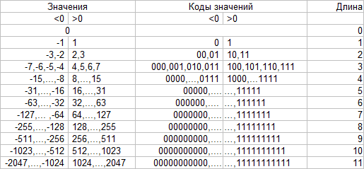
That is, positive values are directly encoded by their binary representation, and negative values are the same, but with replacement of leading 1 by 0. It remains to decide how to encode lengths. Since there are 12 possible values, you can use 4 bits to store the length. But here it is better to use Huffman coding.
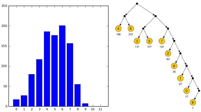
Values with lengths of 4 and 6 are the most, so they got the shortest codes (00 and 01).
JPEG implementation features:
The question may arise: why on the example of the value 9 the code is 1111110, and not 1111111? After all, you can safely raise "9" to a higher level, next to "0"? The fact is that in JPEG it is impossible to use a code consisting only of units - such code is reserved.
There is another feature. Codes obtained by the described Huffman algorithm may not match bits with codes in JPEG, although their lengths will be the same. Using the Huffman algorithm, get the length of the codes, and the codes themselves are generated (the algorithm is simple - start with short codes and add them in turn to the tree as far as possible to the left, preserving the prefix property). For example, for the tree above, the list is kept: 0,2,3,1,1,1,1,1. And, of course, a list of values is stored: 4,6,3,5,7,2,8,1,0,9. When decoding, codes are generated in the same way.
Now order. We figured out how DC is stored:
[Huffman code for DC diff length (in bits)] [DC diff ]
where DC diff = DC current - DC previous
We look AC:
Since the graph is very similar to the graph for DC differences, the principle is the same: [Huffman code for AC length (in bits)] [AC]. But not really! Since the scale is logarithmic, it is not immediately noticeable that the zero values are about 10 times greater than the values of 2 - the next in frequency. This is understandable - not everyone experienced quantization. Let us return to the matrix of values obtained at the quantization stage (using the FastStone quantization matrix, 90%).
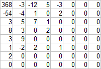
Since there are many groups of consecutive zeros, the idea is to record only the number of zeros in the group. This compression algorithm is called RLE (Run-length encoding, retransmission coding). It remains to find out the direction of bypassing the "consecutive march" - who is behind whom? Writing from left to right and from top to bottom is not very effective, since non-zero coefficients are concentrated near the upper left corner, and the closer to the lower right angle, the more zeros.
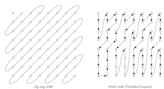
Therefore, in JPEG, an order called “Zig-zag” is used; it is shown in the left figure. This method well identifies groups of zeros. In the right figure - an alternative way to work around, not related to JPEG, but with a curious name ( proof ). It can be used in MPEG when compressing interlaced video. The choice of the traversal algorithm does not affect the image quality, but may increase the number of coded groups of zeros, which may ultimately affect the file size.
Modifying our record. For each non-zero AC - coefficient:
[Number of zeros before AC] [Huffman code for AC length (in bits)] [AC]
I think that you immediately say - the number of zeros is also perfectly encoded by Huffman! This is a very close and good answer. But you can optimize a little. Imagine that we have a certain coefficient AC, before which there were 7 zeros (of course, if written out in a zigzag order). These zeros are a spirit of values that did not withstand quantization. Most likely, our coefficient was also badly battered and it became small, and, therefore, its length was short. This means that the number of zeros before AC and the length of AC are dependent values. Therefore, write this:
[Huffman code for (Number of zeros before AC, length of AC (in bits)] [AC]
The coding algorithm remains the same: those pairs (the number of zeros before AC, the length of AC), which are often found, will receive short codes and vice versa.
We build a histogram of the dependence of the number of these pairs and the Huffman tree.
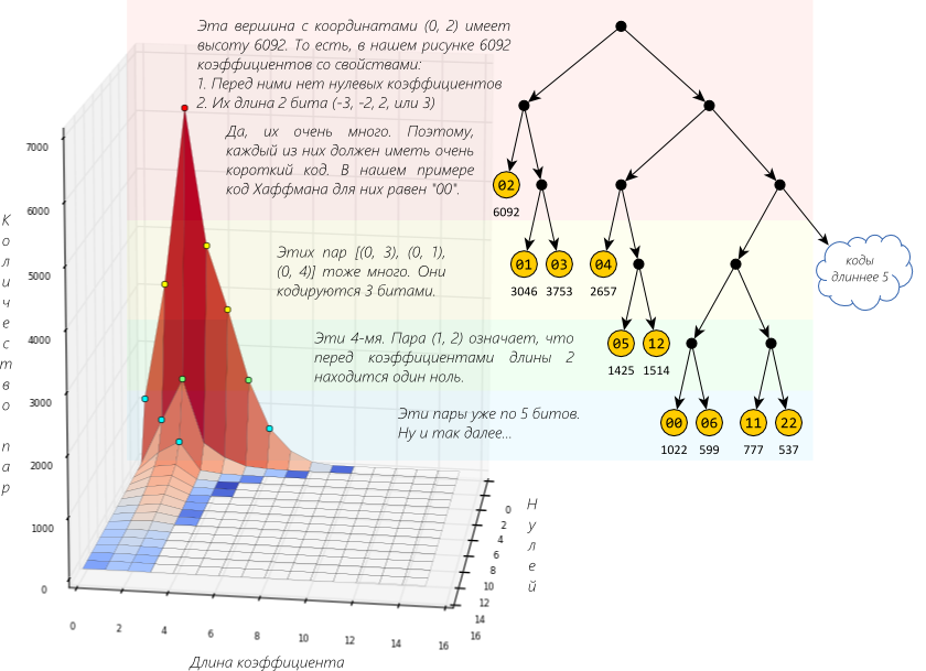
The long "mountain range" confirms our assumption.
JPEG implementation features:
This pair is 1 byte: 4 bits for the number of zeros and 4 bits for the length of AC. 4 bits are values from 0 to 15. For AC, there is enough excess, but can there be more than 15 zeros? Then more pairs are used. For example, for 20 zeros: (15, 0) (5, AC). That is, the 16th zero is encoded as a non-zero coefficient. Since near the end of the block is always full of zeros, then after the last non-zero coefficient a pair (0,0) is used. If it occurs during decoding, then the remaining values are 0.
Found out that each block is encoded stored in a file like this:
[Huffman code for DC diff ]
[DC diff ]
[Huffman code for (number of zeros before AC 1 , length AC 1 ]
[AC 1 ]
...
[Huffman code for (number of zeros before AC n , length AC n ]
[AC n ]
Where AC i - non-zero AC coefficients.
Color image
The way a color image is displayed depends on the selected color model. A simple solution is to use RGB and encode each color channel of the image separately. Then the coding will not differ from the coding of the gray image, only the work is 3 times more. But image compression can be increased if we recall that the eye is more sensitive to changes in brightness than colors. This means that the color can be stored with more losses than the brightness. RGB has no separate brightness channel. It depends on the sum of the values of each channel. Therefore, the RGB-cube (this is a representation of all possible values) is simply “put” on the diagonal - the higher, the brighter. But this is not limited - the cube is slightly pressed laterally, and it turns out rather a parallelepiped, but this is only to take into account the features of the eye. For example, it is more susceptible to green than blue. So there was a model YCbCr.
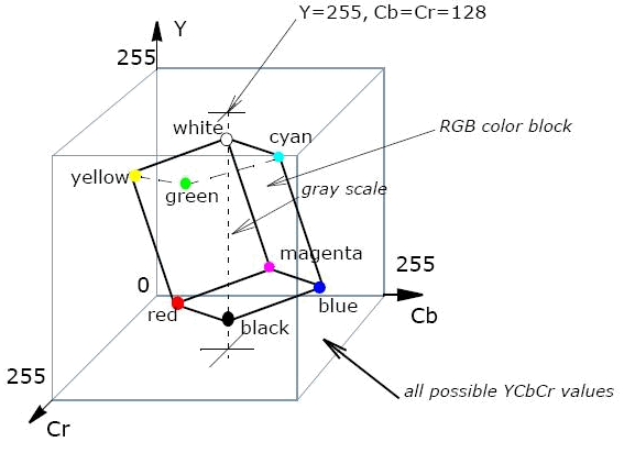
(Image from Intel.com)
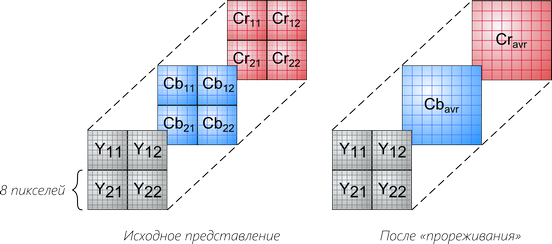
Y is the luminance component, Cb and Cr are the blue and red color difference components. Therefore, if they want to compress the image more strongly, then RGB is transferred to YCbCr, and the Cb and Cr channels are punctured. That is, they break into small blocks, for example 2x2, 4x2, 1x2, and average all values of one block. Or, in other words, reduce the image size for this channel by 2 or 4 times vertically and / or horizontally.
Each 8x8 block is encoded (DCT + Huffman), and the encoded sequences are written in this order:
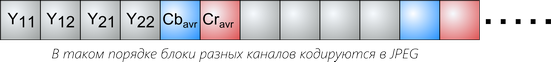
It is curious that the JPEG specification does not limit the choice of model, that is, the implementation of the encoder can arbitrarily divide the image by color components (channels) and each will be saved separately. I am aware of the use of Grayscale (1 channel), YCbCr (3), RGB (3), YCbCrK (4), CMYK (4). The first three are supported by almost everyone, but with the latest 4-channel there are problems. FastStone, GIMP support them correctly, and the regular Windows programs, paint.net,
If they differ in color, or only one picture is visible, then most likely you have IE (any version) (UPD. In the comments say “or Safari”). You can try to open the article in different browsers.
And something else
In a nutshell about additional features.
Progressive mode
We decompose the obtained tables of DCT coefficients into the sum of the tables (approximately like this (DC, -19, -22, 2, 1) = (DC, 0, 0, 0, 0) + (0, -20, -20, 0, 0) + (0, 1, -2, 2, 1)). First, we encode all the first addends (as we have learned: Huffman and zigzag bypass), then the second ones, etc. This trick is useful with a slow Internet, because at first only the DC coefficients are loaded, which are used to construct a rough picture with 8x8 pixels. Then rounded AC coefficients to clarify the figure. Then rough amendments to them, then more exact. Well, and so on. The coefficients are rounded, since in the early stages of loading accuracy is not so important, but rounding has a positive effect on the length of the codes, since each stage uses its own Huffman table.
Lossless mode
Lossless compression. DCT no. The 4th point prediction using three adjacent points is used. Prediction errors are encoded by Huffman. In my opinion, used a little more than ever.
Hierarchical mode
The image creates several layers with different resolutions. The first coarse layer is encoded as usual, and then only the difference (image refinement) between the layers (pretends to be a Haar wavelet). DCT or Lossless is used for encoding. In my opinion, it is used a little less than never.
Arithmetic coding
The Huffman algorithm creates optimal codes for the weight of characters, but this is true only for a fixed correspondence of characters with codes. Arithmetic does not have such a tight binding, which allows the use of codes as if with a fractional number of bits. It is alleged that it reduces the file size by an average of 10% compared with Huffman. Not common due to patent issues, not supported by all.
I hope that now you understand the JPEG algorithm intuitively. Thanks for reading!
UPD
vanwin suggested specifying the software used. I am pleased to announce that everything is available and free:
- Python + NumPy + Matplotlib + PIL (Pillow) . The main tool. Found on the issuance of "Matlab free alternative". Recommend! Even if you are not familiar with Python, then after a couple of hours, learn how to make calculations and build beautiful graphics.
- JpegSnoop . Shows detailed information about the jpeg file.
- yEd . Graph editor.
- Inkscape . He did illustrations in it, such as an example of a Huffman algorithm. I read a few lessons, it turned out very cool.
- Daum Equation Editor . I was looking for a visual formula editor, as I’m not very friendly with Latex. Daum Equation - plugin for Chrome, seemed to me very convenient. In addition to the mouse, you can edit Latex.
- FastStone . I think it is not necessary to represent him.
- Picpick . Free alternative to SnagIt. He sits in the tray, a screenshot that will say where they say. Plus all sorts of buns, such as ruler, pipette, protractor, etc.
Source: https://habr.com/ru/post/206264/
All Articles