Finding the best position when comparing digitized images

The article describes the task of comparing digitized (scanned) images.

A theoretical solution is given to the problem of finding a parallel transfer of a reference image, in which its coincidence with the test image is maximal. We describe computational experiments related to the analysis of shifts of digital digitized symbols. A comparison is made of the constructively computed boundary of a possible shift of one graphic image relative to another and real shifts when considering the class of binary digitized symbols.

Introduction

In many recognition algorithms, two binary images are compared using some proximity function to see if they are images of two “identical” objects. The proximity function is chosen to meet the requirements of the recognition algorithm and take into account the features of the images obtained from a given source.

We consider the space of images U , represented in the form of matrices R = || r _ij || of the same size 0 ≤ i ≤ m , 0 ≤ j ≤ n . The dimensions of the real image are substantially smaller than the dimensions of the matrix n . Placing an image with dimensions of m ₁ n ₁ ( m ₁ < m , n ₁ < n ) in the matrix with dimensions m n is called centering. If the real image is represented by the matrix m ₁ n ₁ , it is possible, for example, to center this image so that the centers of the matrices m ₁ n ₁ and m n matched. It is possible to invent and apply other methods of centering, for us it is important that the method of centering is the same for all images.
')
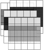
When clustering images and recognizing them, a non-negative proximity function d is used , which compares two images A = || a _ij || and B = || b _ij ||, A U , B U. Conventionally, we will call image A reference , and B - tested . When obtaining images using digital devices (scanners, cameras and camcorders), a number of digitization effects occur. The simplest of these effects is that from a single pre-image can be obtained images that differ both with each other and with the pre-image. This is due to the randomness of the alignment of the pre-image and the digital grid (for example, the scanner grid) and is illustrated by Figure 1 , which shows how two different digitized binary images (black lines) are obtained from a single initial type (the gray band).

Figure 1 - Examples of digitizing the image with a different overlay on the grid scanner
(gray stripes - types, black - binary images)

The proximity function d used in clustering and recognition has two requirements:

• identity axiom - d ( A , B ) = 0 A = B ;
• symmetry axiom - d ( A , B ) = d ( B , A ) A , B.

The contribution of digitization effects when comparing binary images is eliminated (minimized) by choosing the proximity function and applying the shift procedure. In the present paper, Hamming metric is considered as a proximity function.

.

When comparing the images of A and B from the space U, we will perform all possible shifts of the image A = || a _ij || in different directions and consider the proximity function between the resulting image and B. We define the shift of the matrix A by the value of ( h , w ) as



In other words, A ( h , w ) is obtained from A as a result of transferring to the vector ( h , w ) on the torus, which is the closure of the region of a rectangle with dimensions m n (see figure 2 )

Figure 2 - Examples of transferring the image of the symbol "m" to different vectors on the torus

Now we can define the “distance” d ₀ between images A and B.

(one)

The matrix, A ( h , w ) on which the minimum is reached, will be called the optimal position of the image of A with respect to B , and the vector ( h , w ) will be called the optimal shift.

There are various ways to determine d ₀ ( A , B ) and optimal shift ( h , w ).
One of the simplest is to calculate the proximity function d ( h , w ) = ( A ( h , w ), B )), limiting the values ​​of h and w : h ≤ n ₀ , w ≤ n ₀ .

Generally speaking, the smallest value n ₀ that guarantees the achievement of a real minimum d ( h , w ) is not known in advance; the upper limit n ₀ is determined by the amount of shift at which images A and B do not intersect, that is, a _ij b _ij = 0 i and j. For such n _{0, the} method of determining d ₀ ( h , w ) is exact. With values ​​of n ₀ that do not guarantee the achievement of a real minimum d ( h , w ), the method of determining the optimal position is approximate and allows you to calculate d ₀ ( A , B ) with some error.

We believe, however, that the initial position of the image A , which is usually not chosen by chance, should not be too far from the optimal one. Slightly more precisely, if the position taken at random is successful, i.e. if the mismatch of the reference and test images ( A , B ), is a small part of the reference image, then the parallel transfer ( h , w ), which maximizes image matching, is small (i.e., the length is a small part of the diameter of the reference image).

Actually, it is this effect that is the rationale for the restriction of the considered vectors ( h , w ).
It is clear that the smaller n ₀ , the less time the calculation will take d = min _{h, w} d ( h , w ), but I would like to have some estimates of the effect of the shift when comparing two images and, thus, assessing the proximity of the position of some image to the optimal. Obtaining such assessments is devoted to this work.

The first section, which is the development of the work, gives a theoretical analysis. In the second section, experiments on objects of one of the popular recognition tasks are symbols of the Russian alphabet.

1. The study of the effects of shifts when comparing

1.1. Task Description

Below is a mathematical model explaining the above effect at a qualitative level. At the same time, we will significantly expand the original productions. In the model, the image is considered as a pair consisting of the set I (non-zero points of the image), and density φ: I → R (distribution of the weights of the points of the image). The degree of coincidence of the image with densities φ ₁ and φ _{2 is} modeled by the integral .

Let be Is the space with the measure d σ and X is the set of pairs x = ( I , σ), where I - a measurable subset and φ: I → R integrable non-negative function, called density . The metric is defined on the set X where

Let γ: → one-to-one mapping preserving measure, i.e. γ * d σ = d σ. The mapping γ induces isometry taking x = ( i , φ) to a point . By subset and number define a subset of Y X consisting of points ( I , φ) such that:

1. I
2. 

Task 1. For function find the (best) lower score.

One of the possible answers to task 1 is outlined in the next paragraph.
Let us dwell on one modification of problem 1.

Expand the set X and define the set consisting of pairs in which the density φ can be concentrated in points. More precisely, in the set as densities, we consider generalized densities φ, which are sums of integrable functions and finite linear combinations of δ-functions at the points q (we will denote them by the symbol δ _q ), i.e. . On space distance definitions, mappings are automatically transferred and the functions ε, which we will denote, respectively, and . Let the mapping γ be given: → , subset and number . Let the subset consists of points where such that:

1. I ,
2. φ ≥ 0, ≥ 0, the carrier of the function φ lies in I and q _k I ,
3. ;

Task 1 '. For function find the (best) lower score.

1.2. Partial solution of task 1

The following theorem is valid.

Theorem 1. If for some integer n the set is γ ⁿ ( ) does not intersect with the set then .

Evidence. With point y Y we associate a sequence of y ₀ , y ₁ , ..., y _n points in X defined by the relations

Let y = ( I , φ). Since y Y then .

therefore
.

Since the mapping is an isometry, then for any k we have .

By the triangle axiom those. . Q.E.D.

We show that, under certain additional conditions, the estimate from Theorem 1 cannot be improved. The main one is the following condition.

Condition : There is a point q such that the points q , γ ( q ), ... γ ⁿ ( q ) are different and all of them, with the exception of the point γ ⁿ ( q ), lie in the set .

Suppose additionally that the set equipped with a topology in which the set open and the mapping γ is continuous.

Theorem 2. Let the conditions listed above and . Then .

Evidence. Choose a point q satisfying the condition and take its neighborhood E of positive measure, so small that for each k = 0, 1, ..., n, the neighborhoods of γ ⁿ ( E ) do not intersect with each other and all of them, except for the neighborhood of γ ⁿ ( q ), lie in set . Let φ ₀ be a non-negative function on whose carrier lies in the domain E , such that .

Let x = ( I , φ) be a point from determined by the following relations:



Then

.

We have

.

Easy to see that

.

Therefore, ε ≤ 2 a / n . By Theorem 1, ε ≥ 2 a / n . Theorem 2 is proved .

Partial solution of the problem 1 ' . Theorem 1 is literally generalized to the case of problem 1 '. We will not dwell on the formulation and proof of this generalization. Theorem 2 for the case of problem 1 'admits a strengthening: it is not necessary to additionally require that the set was equipped with a topology in which many open and the mapping γ is continuous.

Theorem 2 '. Let the condition be fulfilled and . Then .

For the proof, it suffices to consider the point equal to the set of points endowed with densities equal to δ-functions multiplied by / n . The further proof of Theorem 2 'is similar to the proof of Theorem 2.

1.3. The case of Euclidean space

Let space with measure d σ is the space R ⁿ with a Euclidean measure, the map γ is a shift by a fixed vector a R ⁿ (i.e., γ ( x ) = x + a ), and the set this is any n- dimensional convex subset in R ⁿ . Consider a set of nonnegative integrable functions φ in R ⁿ , identically equal to zero outside a convex set and satisfying the relationship:



Problem 1 for Euclidean space. Find the (best) lower estimate of the function ε ( , , a) given by the formula:



Task 1 'in the case under consideration is formulated similarly.

Vector a R ⁿ we will write in the form a = | a | ν, where ν is a vector of unit length and | a | - the length of the vector a . For a vector of ν of unit length, we call ν- diameter d _v ( a) convex figure the exact upper bound of the set of lengths of segments that are sections of the region straight lines parallel to the vector ν. For a nonzero vector a = | a | ν is called a-diameter d _a ( a) convex figure ratio d _v ( ) / | a | its ν-diameter to the length | a | vector a .
We present the solution of problems 1 and 1 'for the vector a = | a | ν in the case when a is the diameter of a figure is not a natural number.

Theorem 3. If for some integer n ≥ 0, the inequalities n | a | <d _v ( ) <(n + 1) | a, then ε = 2 / (n + 1).

Evidence. Under the conditions of Theorem 3, we have . Therefore, according to Theorem 1, the inequality ε ≥ 2 / ( n + 1). Since the exact upper bound of the section lengths is straight lines parallel to the vector ν are greater than the number n | a |, then there is a point y lying strictly inside the region , such that all points y , y + a, ..., y + na lie strictly inside . By Theorem 2, we have ε ≤ 2 / ( n + 1), whence Theorem 3 follows.

We present the solution of problem 1 'for the vector a = | a | ν in the case when a is the diameter of a figure is a natural number.

Theorem 4. If for some integer n ≥ 0, the equality n | a | <d _v ( ), then .

The proof of Theorem 4 is similar to the proof of Theorem 3. If the equality n | a | < d _v ( ), then the minimum in the problem is not achieved on ordinary functions. However, the minimum is reached on a linear combination of δ-functions, and it is equal to 2 / ( n + 1).

1.4. Implications of the ratings found

The formula for the function ε ( , , a ), rather cumbersome. In Corollary 1, an inaccurate, but fairly good estimate of this function is given, which is quite observable. In Corollary 2, we give an estimate of this function, which for a fixed vector ν for small values ​​of the length | a | linear in length | a |, i.e. equal to λ | a | with explicitly written constant λ.

Corollary 1. Fair assessment



This estimate is exact for | a | = d _v ( ), d _v ( ) / 2, d _v ( ) / 3,… and as | a | → ∞ (i.e., figuratively speaking, is exact when | a | = d _v ( ) / 0).

If ε ( , a) <2 then this inequality can be rewritten in the form:



Corollary 2. For any y ₀ ≥ 0 with 0 ≤ | a | a | ≤ y ₀ we have



with | a | ≥ y ₀ we have



In particular, for y 0 = d _v ( ) we get the following: for 0 ≤ | a | ≤ d _v ( ) we have



with | a | > d _v ( ) we have ε ( , , a) ≥ (note that in fact, with | a |> d _v ( ) the equality ε ( , , a)) = 2 ).

Evidence. Corollary 1 automatically follows from Theorems 3 and 4. Corollary 2 follows from Corollary 1.

1.5. Qualitative explanation of the effect under consideration

Let φ (x) be a non-negative integrable function on R ⁿ equal to zero outside a convex set . Let be



Let g (x) be another non-negative integrable function on R ⁿ . Let be

(2)

Assume that the integral significantly less than .

Task 2. Changing the parameter a R ⁿ , ensure that the integral

took the least possible value.

Our goal is to show that if >> , then to minimize the numbers ψ ( a ) only the small a along the vector a = | a | ν, which are significantly shorter than the ν-diameter d _v ( ) areas .

We define the function ε ( a ) as

where the minimum is taken over all non-negative functions φ satisfying relation (2) and having a carrier in the region .
We can apply the estimates of the function ε ( a ) found above.

Theorem 5. We fix a vector ν of unit length. Let d (ν) be a minimal number such that for the vector a = | a | ν, for | a | > d (ν) the inequality ε (a)> 2 holds .
Then for | a | > d (ν) the inequality holds

.
In particular, to minimize ψ (a), it suffices to consider only the vectors a = | a | ν, for which | a | <d (ν) .

Evidence. It follows from the triangle axiom. Indeed, we have


Where at | a |> d (ν)

, as required.

Corollary 3. To minimize the integral ψ (a) on the line a = | a | ν, spanned by the vector ν, it suffices to consider only the vectors a for which the inequality holds

(3)

With fair inequality

.

Evidence. It follows from Theorem 5 and Corollary 1.

Corollary 3 provides a qualitative explanation of the effect under discussion. Indeed, if >> then the number / ( - ) few. Therefore, the minimum ψ ( a ) is achieved when the length of the vector a is much smaller than the diameter d _v ( ) figures in the direction of the vector ν. It was thus proved that in order to achieve the “optimal” position of two figures, small enough shifts in the case when the measure of mismatch at small shifts is insignificant.

2. Experiments

2.1. Source objects, parameters and algorithms

The proved theorems give a constructively calculated boundary of the possible shift of one graphic image relative to another in order to obtain the minimum distance. It is interesting to understand what real shifts will be obtained when considering a particular class of objects. We present the results of experiments in which printed characters taken from the scanned image of the page of a regular book appeared as objects.

So, the source material is a test set consisting of 1770 images of letters of the Russian language. Different pairs of signs are considered, totaling 1770 (1770–1) / 2 = 1565565 pairs.

We will use the AL ₁ algorithm to set the initial (zero) position of the two images A ₁ and A ₂ relative to each other. The value of the proximity function based on the Hamming metric in this position will be denoted ( A ₁ , A ₂ ). In addition, we will consider the optimization algorithm AL ₀ . This algorithm enumerates various parallel translations of one of the images on all possible vectors ( h , w ) with respect to the initial position and selects the one at which the Hamming metric takes the minimum value. This (optimal) value will be denoted by d ₀ ( A ₁ , A ₂ ) and the optimizing vector ( h , w ) by a ( A ₁ , A ₂ ) = | a | ν, where ν is the unit direction vector. Usually we will consider the value n ( A ₁ , A ₂ ) = [ a ( A ₁ , A ₂ )], which characterizes the distance between the zero and optimal position in pixels.

The number of nonzero pixels of the image A will be denoted . As shown in the previous section, the relation plays an important role. / . In this case, since in all cases when it comes to a pair of images A ₁ and A ₂ , the values / ₁ and / ₂ act symmetrically, we will consider the value of t ( A ₁ , A ₂ ) = min ( / ₁ , / ₂ ).

This, in particular, “symmetrizes” the formulas of p. 1.5, related to the functions φ (x) and g (x).
This also saves us from having to consider large values. / , as always t ≤ 2. The corresponding value in the optimal position will be denoted by t ₀ :

t ₀ ( A ₁ , A ₂ ) = min ( d ₀ / ₁ d ₀ / ₂ ).

Finally, we note that in statistical tables, and also where it does not lead to confusion, we will omit the arguments A ₁ and A ₂ and write simply , d ₀ , t , t ₀ , n .

2.2. General characteristics

Among the considered 1770 images of the characters of the Russian alphabet, some are of the same name (for example, the letters " in "). It is clear that many of the characteristics for such pairs can differ greatly from the corresponding characteristics of the “opposite” pairs. Therefore, sometimes we will consider statistics on such pairs separately.

In cases where the number of pairs with some property is plotted along one of the axes, the maximum values ​​may be large, but it is important for us to see small values. In such cases, we will use the logarithmic scale: n → log ₂ ( n +1).

Let us turn to statistics. First of all, let us show the total distribution of the number of pairs over various values ​​of t ₀ and t . Figure 3 shows the histogram of the dependence n ( t ₀ ) and n ( t ) for all pairs of symbols.

a)

b)

Figure 3 - The total number of pairs depending on a) t ₀ , b) t

We add that the average value of t ₀ for all pairs is 0.6, the average value of t is 0.66.

Consider in Figure 4 a similar histogram for pairs of the same name.

a)

b)

Figure 4 - The number of pairs of like symbols depending on a) t ₀ , b) t

Here, the average value of t ₀ for all pairs is 0.17, the average value of t is 0.23.

On average, the AL ₁ algorithm gives values ​​that are not very far from optimal. For pairs of the same name, in the right-hand part of the graph, the values ​​of n ( t ) fall much less steeply towards zero than n ( t ₀ ). This means that large values ​​of t do not always indicate that the corresponding optimal value of t ₀ is large.However, for small values ​​of t ₀ and t, both graphs behave approximately the same.

Note that, both from the point of view of applying Theorem 5, and in the context of recognizing a pair with large t ₀ (for example, t ₀ > 0.5), we are of little interest, therefore, the quality of the AL ₁ algorithm and the search for the optimal shift are not too important .

In addition, we consider in Fig. 5 a histogram of the number of pairs depending on the value of t ₀ / t .

Figure 5 - The dependence of n ( t ₀ / t )

As we can see, more than 15% of all considered pairs are obtained using the AL ₁ algorithm , differing from the best possible (ideal) by no more than 1%, and then their number decreases monotonically with t ₀ / t .

Thus, it can be assumed that the shift statistics obtained by comparing the position determined by the AL ₁ algorithm with the optimal position ( AL ₀ algorithm ) will be quite representative.

2.3. Analysis of deviations of the initial position from the ideal

Consider the deviation from the ideal position depending on t in more detail. On Figure 6 shows the number of pairs of n _i , deviating the zero position from the ideal position to i = 0, 1, 2, 3, and 4 i > 4, as a function of t .

Figure 6 - The number of pairs n _i ( t ) deviating from the ideal position by i pixels, as a function of t ( n ₅ ( t ) - the number of pairs with i > 4)

It is clear from the graph that for t <0.13 all pairs of characters are ideally located, but already at t > 0.22 the number of pairs requiring a shift by 1 pixel exceeds the number of ideally arranged ones. And only at t > 0.3 pairs appear, requiring a shift of 2 pixels.

Pixel deviation / t	0	one	2	3
0.0 - 0.12	4344	0	0	0
0.12 - 0.31	32158	34271	0	0
0.31 - 0.38	42	8809	38	0
0.38 - 0.49	0	3328	522	0
0.49 - 0.66	0	241	463	0
0.66 - 0.85	0	0	31	7

Table 1 - Distribution of quantities of pairs of the same name with different deviations of the initial position from the ideal

In this case, we note that although the algorithm for determining the initial position, as already noted, is not bad, the dependence on t is significant here, as Table 1 shows .

It gives the number of pairs in which the deviation of the initial position from the ideal is i = 0, 1, 2 and i > 2 for the symbols of the same name. We see that even here there are not a few cases when the initial position is far from ideal, but they all refer to rather large values ​​of t .

So far, we have used the specific algorithm AL ₁ for comparison with the ideal.. Now we will consider how the theory “in its pure form” works in our experiment. Namely, each pair of characters is shifted relative to the ideal position in all directions, first by 1 pixel, then by 2, 3, and 4, and in each case we consider the minimum deviation in all directions. So we will see what is the minimum value / when the deviation from the ideal value | a | (| a | = 1, 2, 3 and more than four pixels) for all 1565565 pairs of characters available. In addition, for each | a | calculate the minimum value of S _v by the formula (3) .

When | a | = 1 for t ₀ > 0.12 there is always a pair for which a shift by one pixel in any direction does not change the value of t . Oddly enough, for other values ​​| a | such examples are also found, but only for t ₀ > 0.5, which go beyond the theoretical estimates (recall the assumption of Corollary 3: << ).The results of the experiment are shown in table 2 .

| a |	min /	min S v
one	0.12	2.32
2	0.28	5.81
3	0.44	8.94
four	0.51	11.18

Table 2 - The minimum values ​​of β / α and S _v when the deviation from the optimal position by 1, 2, 3, 4 or more pixels

The data in Table 2 well confirm the theoretical conclusion. Having obtained the value t <0.28, we can confidently assert that the optimal position is no more than two pixels. And even at t = 0.43 (the distance is approximately equal to half of the character area), the mutual position differs from the ideal one by no more than three pixels.

At the same time, it is clear that the theoretical estimate | a | < S _v is weak. The value of S _v everywhere several times exceeds the real shift from the optimal position.

findings

We considered the comparison of binary raster images, taking as a measure of proximity - Hamming distance between them. It was proved that if it is sufficiently small, then the parallel transfer a = ( h, v ) of one of the objects, which minimizes the value , also cannot be large. A constructive estimate of S _v for | a |

In the considered experiment with the images of symbols, the theoretical results are fully confirmed. However, the theoretical value of the boundaries of a possible shift Sv is somewhat overestimated in relation to real shifts, which is not surprising in view of the very general theoretical premises and the roughness of the estimates.

The full text of the article was published in “Arlazarov V.L., Slavin O.A., Farsobina V.V., Khovansky A.G. The search for the optimal position when comparing digitized images of characters // Artificial Intelligence and Decision Making, V.3. M .: Poliprint Service, 2013. P. 48-59 "

Literature

1. Zhuravlev Yu. I., Ryazanov V.V., Senko O.V. “Recognition”. Mathematical methods. Software system Practical applications. - M .: Fazis, 2005. - p. 176. ISBN 5-7036-0108-8.
2. Arlazarov V.L., Kotovich N.V., Slavin O.A. Adaptive recognition // Information technologies and computing systems. - 2002, № 4. - p. 11-22. ISSN: 2071-8632.
3. Arlazarov V.L., Slavin O.A., Khovansky A.G. Estimation of the distance between images with parallel transfer // Reports of the Academy of Sciences. - 2011, T. 437, No. 3. - p. 313-315. ISSN: 0869-5652