Bresenham algorithm in real-time applications

There are such devices - they are called scanners or scanners, usually with the adjective "laser"



use them in various laser scanning technologies.
')
From the programmer's point of view, a laser scanner is two rotating mirrors that deflect a laser beam in two mutually perpendicular planes, the angles are set using a pair of DACs (and feedback amplifiers after DACs). Usually DACs can be 12-16 bits. In fact, the task of drawing a picture or, in a slightly more scientific language, the output of information on such a device is no different from the output of information on ancient analog graphic displays.



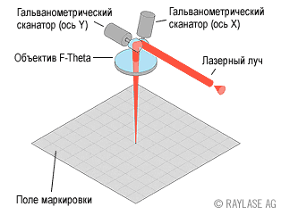
Such scanners are usually controlled using a separate (micro) controller, to which “high-level commands” are sent from the computer. The main team is “draw a line from now to this with such a speed”. Once “draw a line” and a microcontroller, we recall the classic Bresenham algorithm. The Bresenham algorithm is good in that it does not use any "slow" floating-point operations, although for modern 32-bit microcontrollers this is not as important as for 8 or 16-bit ones.

/* Bresenham algorithm implementation   .. , .. ,  ,*/ void Line(int x1, int y1, int x2, int y2, int color) { int x1,y1,dx,dy,sx,sy,d,d1,d2; int i, x,y; if( x2 >= x1) { dx = x2 - x1; sx = 1; } else { dx = x1 - x2; sx = -1; } if( y2 >= y1) { dy = y2 - y1; sy = 1; } else { dy = y1 - y2; sy = -1; } if(dy <= dx) { d = (dy << 1) - dx; d1 = dy << 1; d2 = (dy - dx) << 1; for(x=x1+sx,y=y1,i=1; i <= dx ; i++,x+=sx) { if(d > 0) { d += d2; y += sy; } else { d += d1; } putpixel(x,y, color); } } else { d = (dx << 1) - dy; d1 = dx << 1; d2 = (dx - dy) << 1; for(x=x1,y=y1+sy,i=1;i <= dy ; i++,y += sy) { if(d > 0) { d += d2; x += sx; } else { d += d1; } putpixel(x,y, color); } } /* endif(dy <=dx) */ } 

In our case, there is no color, so we ignore color . But we have speed.
For example, if we have a horizontal or vertical segment of n pixels and the given speed is V (pixels per second), then each pixel should display the time tp = 1 / V

If the segment is not horizontal, then its length is l = hypot (x0-x1, y0-y1) , the output time of the entire segment is t0 = l / V , but to calculate the delay per point, it will be necessary to divide t0 by the number of function calls putpixel, t. e.

tp = t0 / max (| x0-x1 |, | y0-y1 |)

Then in the algorithm, the color is simply replaced by “delay by point” wait (= tp)

 void Line(int x1, int y1, int x2, int y2, int wait) ...... putpixel(x,y, wait)); 

at first glance, the putpixel function itself should look something like this

 void putpixel(int x, int y, int wait)) { outPortX(x); //    X  x outPortY(y); //    Y  y delay(wait); //  wait   } 

However, here begin the nuances associated with the implementation of the DAC.

DACs can work both in series and in parallel. Consistently - when you need to choose the number of the DAC, set the desired value and wait for the readiness, the end of the conversion, or just wait for a while. If DACs work in parallel, then you can write the values ​​of x and y in the corresponding registers of the microcontroller, and then simultaneously wait for the readiness or the end of the conversion.

In the first case, the time spent on outputting only X or only Y is approximately two times less than the serial output of X and Y. Accordingly, the source code looks like this

 void Line(int x1, int y1, int x2, int y2, int wait, int waitXY) { int dx,dy,sx,sy,d,d1,d2; int i, x,y; if( x2 >= x1) { dx = x2 - x1; sx = 1; } else { dx = x1 - x2; sx = -1; } if( y2 >= y1) { dy = y2 - y1; sy = 1; } else { dy = y1 - y2; sy = -1; } /****************************/ if(dy <= dx) { d = (dy << 1) - dx; d1 = dy << 1; d2 = (dy - dx) << 1; for(x=x1+sx,y=y1,i=1; i <= dx ; i++,x+=sx) { if(d > 0) { d += d2; y += sy; putXY(x,y,waitXY); } else { d += d1; putX(x, wait); } } } else { d = (dx << 1) - dy; d1 = dx << 1; d2 = (dx - dy) << 1; for(x=x1,y=y1+sy,i=1;i <= dy ; i++,y += sy) { if(d > 0) { d += d2; x += sx; putXY(x,y,waitXY); } else { d += d1; putY(y, wait); } } } /* endif(dy <=dx) */ } void putXY(int x, int y, int wait)) { outPortXY(x,y); //    X  Y  x  y //    #define outPortXY(x,y) outPortX(x); outPortY(y); delay(wait); //  wait   } void putX(int x, int wait)) { outPortX(x); //    X  x delay(wait); //  wait   } void putY(int y, int wait)) { outPortY(y); //    Y  y delay(wait); //  wait   } 

The wait and waitXY values when calling Line can be calculated based on the fact that:

l = hypot (x0-x1, y0-y1) , the output time of the entire segment t0 = l / V , the number of calls to putXY n1 = min (| x0-x1 |, | y0-y1 |), the number of calls to putX or putY n0 = max (| x0-x1 |, | y0-y1 |) - min (| x0-x1 |, | y0-y1 |) .

In addition, you can enter a correction for the execution time of the functions outPortX, outPortY and outPortXY. The execution time of these functions can be predetermined during the calibration process.

Let me remind you that all the delay calculations we do in the control computer, not in the microprocessor, and the times and delays in question are microseconds and their shares ...

Well, actually all for now.

We assemble the installation, write programs for the control computer and the microprocessor, turn it on, display some simple test image and look at what happened

Anyone guess what we will see? (to be continued)