Linear regression on fingers in recognition

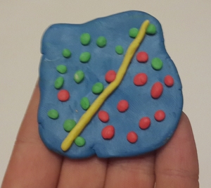In the task of recognition, the key role is played by the selection of significant parameters of objects and the evaluation of their numerical values. Nevertheless, even having received good numerical data, it is necessary to manage to use them correctly. Sometimes it seems that the further solution of the problem is trivial, and one would like “from general considerations” to obtain a recognition result from numerical data. But the result in this case is far from optimal. In this article I want to show, using the example of the recognition problem, how you can easily apply the simplest mathematical models and thereby significantly improve the results.

About the pattern recognition task

The task of pattern recognition is the task of classifying an object to a certain class. To determine belonging to a class, a certain set of object parameters is used. For example, you can recognize people by some of their parameters: the distance between the eyes, skin color, nose length, iris pattern, characteristic voice frequency, number of fingers, etc. 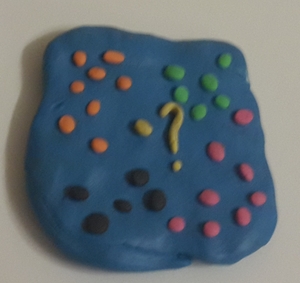These parameters can be represented as a numerical vector of a fixed dimension (for numerical parameters this is trivial, for the color / pattern of the iris / face image, etc., we must also figure out how to do this). That is, we have a certain number of classes X ₁ , X ₂ , ... X _N , there is a prototype, described by a set of parameter values , and we want to say about him if he belongs to one of these classes. Usually classes are presented in the form of several samples of this class: for example, visual images of an object from different angles, various measurements of parameters, and various copies of photographs of the iris. Then the simplest method of recognition is to compare the incoming object with each sample of each class, and by the distance from the nearest object, decide whether it is he or not.

At first glance, the task sounds like a classification task with an indefinitely large number of classes: each type of object is a separate class, and a new object must be compared with each class. 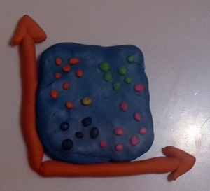This is quite a difficult task, especially when we have an unfixed number of classes: for example, when recognizing people, a person who does not exist in the database can pass - that is, a person of another class. But in fact, we calculate the difference dx between the object under study and the sample class and make a decision, is it the same or different object. For example, if we want to recognize a person by fingerprints, then we compare the resulting fingerprint with all fingerprints from a certain database, calculate the measure of similarity between each pair of fingerprints, and according to this measure of similarity for the most similar fingerprint, decide that this is the same Man, if the prints are similar enough, or that this person is not in our database, if the most similar imprint is still not similar. That is, our classifier takes as input not the parameters of the object x, but the difference between the parameters of two objects dx = x - x ⁱ (it is better to even take the difference module of each component so that the order of subtraction is not important), and by these parameters it gives a characteristic (measure of similarity ), allowing to make a decision: are they the same objects or different. 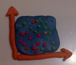This can be viewed as a classification task with two classes: “identical pairs of objects” and “different pairs of objects”. And the class of "identical pairs" will be heaped closer to zero, and different - on the contrary, they will be somewhere aside. Traditionally, the classifier should produce a numerical measure of similarity (for example, from 0 to 1), which is greater, the greater the likelihood that these are different objects; Further, depending on the requirements of the system, a threshold is determined for making a decision, on which errors of the first and second kind depend.

How not to do

Initially, looking at these parameters, I just want to find the norm of the difference vector - the root of the sum of the squares of the components: . That is, as the Euclidean distance between the samples, if the parameters are considered as coordinates. The smaller it is, the more “similar” these two objects are, that is, there is a greater chance that they are the same. This is correct, but with a number of limitations: all parameters must be uncorrelated (mutually independent), they must have the same distribution (they must be equivalent). This is usually not the case (for example, height and weight should not be considered independent, and the shape of the nose is a much more reliable characteristic than the shape of the mouth or the length of the hair). Then let the different components choose different weights to strengthen the more important parameters and weaken the less important ones: .
')
Here we come to a very correct idea: we must take all sorts of factors not from our head, but from practice, that is, we need to choose them so that they work well on some data set. In machine learning, this is called “learning with a teacher” : a set of data is taken (objects of different and identical classes, about which we initially know which class they belong to), called “training set”, and the coefficients are chosen so that our recognizer worked as best as possible (this is called "learning"). Then you can check how well the model works by applying it on another data set, called “test sample”, and conclude how well we did it.

So we want to determine the weights. To do this, we walk through all pairs of objects from the test sample and for each component we calculate its average value and variance for the same pairs and for different pairs. But what to do next with this is not very clear. The weights should be greater, the greater the distance between the average values ​​( ), while still they should be less if the variance is very large, that is, the components are more noise than informative. All my attempts at optimization at this stage led to the need to take one most important component, and not to consider the rest, which obviously will not give a good result. In the end, I scored on the dispersion and just counted for each component , the exponent k was chosen experimentally, and for different sets of parameters the best indicator could turn out to be equal to both 0.01 and 4.

Yes, this method gave much better results than just calculating the norm of the vector. But he has at least two significant drawbacks. The first thing that catches your eye is a formula sucked out of your fingers for weights, which means that we are not talking about any optimality. Well, and secondly, all components are considered separately and independently, that is, they are meant to be uncorrelated, which is generally wrong.

Linear regression

The correct approach is to mathematically formalize the problem and find the optimal solution in some sense. As is known, the simplest function is a linear function, so we will look for a function of the form (yes, it looks very similar to those weights). 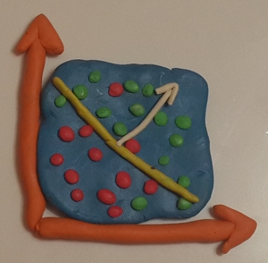Finding such a function is called linear regression. The coefficients b ₀ , b ₁ , ... b _n will be chosen in such a way that this OLS function best suits the correct values ​​for the test sample. And the correct values ​​are Y = 0 for identical objects and Y = 1 for different. Intuitively, it seems that the value of b ₀ must be equal to 0, because on the zero vector of difference we have guaranteed identical objects. But we will not play a guessing game and calculate b ₀ to be honest. Thus, we essentially define the direction in the n-dimensional space in which the same and different pairs will differ most strongly.

(source) The sum of the squares of the errors will be defined as . Hereinafter, M is the number of test sample objects, the superscript denotes the number of the object in the sample, the superscript is the number of the object's components. This error is minimized at the point at which the derivative for each component is zero. Elementary mathematics leads us to the system Ab = f, where A is the matrix (n + 1) * (n + 1), , , , i, k = 1..n. , . We calculate the elements of the matrix by the test sample, we solve the system, we get the coefficients, we build the function.

It may seem strange that some coefficients b _i turn out to be less than zero, that is, as if the more strongly the objects differ in this parameter, the more they are similar. In fact, there is nothing wrong with that, it just says that we have learned the correlation between different parameters (for example, roughly speaking, this parameter only grows with another parameter and compensates for the third one).

My experience shows that such a function distinguishes between identical and different pairs of objects, much better than randomly chosen weights. This is not surprising, because this function is optimal in a certain sense.

Problems?

What problems may arise?

First, to determine the coefficients of the function of n parameters, it is necessary to calculate a matrix of size (n + 1) * (n + 1), that is, all pixels of the image 256x256 cannot be represented as separate parameters, there is not enough memory. Here you can resort to the traditional methods of lowering the dimension, in particular PCA . 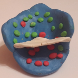Or you can choose a certain number of the most significant parameters (for example, weed out those whose average value for different does not exceed the average value for the same, or the dispersion is too large). And since no one reads the entire article, I propose to select parameters that have the most beautiful numbers, for example, that end in a seven.

Another problem is if linear approximation is not enough, and the function separates classes too poorly. Then you can use more complex classifiers - adaboost , SVM + kernel trick ( article on the topic ), etc.

Another important problem of all “teacher-to-teacher” systems is retraining . Roughly speaking, if we have a lot of different parameters, then when learning we can detect some regularities that we don’t actually have (random fluctuations). Then, when checking outside the training sample, this pseudo-consistency pattern will no longer exist, which will negatively affect the recognition result. Wikipedia has mentioned methods for dealing with this, such as regularization, cross-validation, etc.

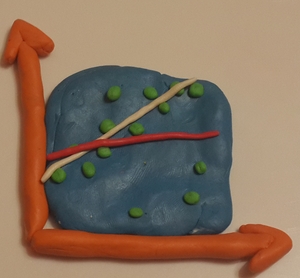
It can also worsen the result of training on a sample with errors. If there are a lot of erroneous values ​​in the training sample, they can significantly affect the final result. Traditionally, this is solved in the following way: training takes place, after which those objects that have produced a big error on this model are thrown out of the training sample. Under the new, “thinned out” learning sample, training is again being conducted. If desired, the procedure can be repeated several times.

findings

Even if you come up with a clever system of matching contours, detecting tails or counting fingers, you will still most likely have a vector of parameters according to which you will need to build an evaluation function and make a decision, and you will still need machine learning. And even the simplest mathematical model gives much better results than “general considerations”, because it is in some way optimal.