Fast, economical, steady ...
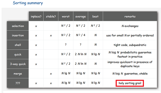
If you need an array sorting algorithm that:
- Would work guaranteed for O (N * log (N)) operations (exchanges and comparisons);
- Would require O (1) additional memory;
- Would be stable (that is, did not change the order of elements with the same keys)
then you will most likely be offered to limit to any two of these three points. And, depending on your choice, you will receive, for example, either merge sorting (requires O (N) additional memory), or pyramidal sorting (unstable), or bubble sorting (works for O (N 2 )). If you weaken the memory requirement to O (log (N)) (“for recursion”), then you will find an algorithm with complexity O (N * (log (N) 2 ) - rather unknown, although it is its version that is used in the implementation method std :: stable_sort ().
When asked whether it is possible to achieve the fulfillment of all three conditions at the same time, the majority will say “hardly”. Wikipedia does not know about such algorithms. There are rumors among programmers that there seems to be something like that. Some say that there is a “stable fast sorting” - but for the implementation I saw, the complexity was still the same O (N * (log (N) 2 ) (by timer). And only in one discussion on StackOverflow they gave a link article BC. Huang and MA Langston, Fast Stable Merging and Sorting in Constant Extra Space (1989-1992) , which describes an algorithm with all three properties.
The authors say that their algorithm is not the first, and refer to the work of L. Trabb Pardo, Stable sorting and merging with 1974 . This is about 80 pages of scanned text, and I did not try to understand it.
')
I will immediately say for those who try to understand the article by Huang and Langston that I failed to implement the algorithm in the form in which it is described there. The technique that they use in clause 4.3 does not work, because the statement " right " is not always true. Fortunately, in some later works we managed to find a way to get around this trouble, and now I can say that an algorithm that satisfies all three conditions really exists.
So, let's begin...
Basic operations
To work with an array, we need functions:
- SWAP1 (A, B) - swap two elements. The difficulty is 1.
- SWAPN (A, B, K) - swap K pairs of elements of arrays A and B. Difficulty is K.
- ROTATE (A, K, L) - rearrange two consecutive fragments of array A, the length of the first is K, the length of the second is L. The complexity does not exceed K + L.
- BinSearchLeft (X, A, L) - find the leftmost place to insert an element X into an ordered array A of length L. Valid result values are from 0 to L. The complexity is log (L).
- BinSearchRight (X, A, L) - find the rightmost place for inserting an element X into an ordered array A of length L. Valid result values are from 0 to L. The complexity is log (L).
We are looking for a clipboard.
First, some terminology.
About the elements for which the comparison function gave the result that they are equal, we will say that "they have the same keys," although physically no keys may exist. Accordingly, it is possible to determine the number of different keys in the array and the elements with different keys.
Two array states will be called equivalent if the elements with the same keys in them are in the same order. The main problem of stable in-place sortings is not to lose this equivalence, or always be able to restore it.
Let the length of the array be N. If N <16, then we will not sort such an array, but call the insertion sort instead, this will not affect the overall asymptotics.
Choose a number S equal to the power of two, close to sqrt (N). Define K = [N / S]. And we will try to find pairs of different keys in the K + S array.
The first idea is that if we take for each key the leftmost element of the array with this key, and collect all such elements at the beginning of the array (preserving the order of the other elements), the equivalence will not be broken, but this will give us the space in which we we can freely rearrange and compare with each other elements.
During the search, we will keep the found keys in a continuous fragment of the array, and move it forward as new keys are found: going through the array elements, we will search the binary search for them in a fragment of the found keys, and if we haven’t found it, we will adjust the array with the keys to the found element, and for the second - put a new element in the right place in this fragment.
Keys are collected in ascending order, which saves time by checking whether we already have an element with the same key as the current element. The number of movements of a fragment with keys is not greater than the number of found keys, so the complexity of this stage is, in the worst case, N * log (NKeys) comparisons and 2 * N + NKeys 2 exchanges. Since NKeys we have about 2 * sqrt (N), so far we have not gone abroad.
Now we have two options. Either we found the ordered K + S keys, or did not find them. These cases are handled slightly differently. In addition, there is a case when the number of different keys is less than 4 - it also has its own processing.
Case A. There are many different keys.
We have K + S different keys collected at the beginning of the array. We will declare the first K of them "keys for marking fragments" and for now we will not touch them. The remaining S will be the buffer for the merge. All remaining elements of the original array are “data”, now they are at the end of the array.
A.1. Stage of classical merge sorting.
Let's write two more functions. One will be called MergeLeft, the other MergeRight. They are fed to the input fragments of arrays, consisting of three parts. In the case of MergeLeft, this is a buffer of length P, a sorted fragment of length Q and a sorted fragment of length R, where S≥R. The function should merge the second and third fragments, put the result at the beginning, and the buffer elements in arbitrary order at the end of the fragment. The MergeRight function works as a mirror — it has two sorted fragments at the input, followed by a buffer, and the output, on the contrary, a buffer, and a sorted fragment after it. It looks like this:

The complexity of both functions does not exceed Q + R - both by comparison and exchanges.
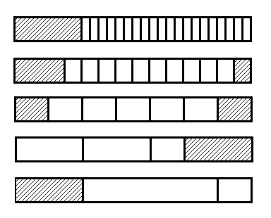
Using the MergeLeft function, we can sort the data first by pairs, then by fours, ... up to fragments of length S (recall that S is a power of two). Every time when sorting M elements we use a piece of buffer of length M / 2, which as a result leaves for the right side of the array. At the pair sorting stage, we will use a piece of the buffer of length 2, so that by the time the sorted pieces are S, the data array will be pressed to the left, and S buffer elements will be on the right. Now we can use MergeRight, sort the fragments of length 2 * S, and at the same time, return the buffer to the beginning.
A.2. Stage block sorting.
Now we have sorted fragments of length G = 2 * S. We will merge them in pairs, then again in pairs, etc., until we reach the size of the entire data array. For this we have a buffer of length S and an array with keys of length K, where K ≤ L / S (L is the total length of the data array).
So, the cycle “for now G ≤ L”.
We want to merge two consecutive fragments of length G, and immediately before them is a buffer of length S (G and S are powers of two). We divide our fragments into blocks of length S. Let them be K 1 . The second fragment at the very end of the array could have a length less than G, and after dividing it may remain an incomplete block, we also consider it (although we will not move). Take the first K 1 keys (they lie at the beginning of the original array), sort them (for example, inserts) and remember the key index with the number G / S (now it is equal to G / S, but then it will change) - let's call it midkey. Each key has its own block. We use them, firstly, to distinguish between the first and second merged fragments, and secondly, to maintain the order of blocks with the same elements. Because now we will mix them as horrible.
We sort the blocks. The order will be determined by the first elements, and if they are equal, then the keys corresponding to these blocks. The only sort we can use here is sorting by choosing the minimum element, since it requires no more than K 1 exchange (and K 1 2/2 comparisons): exchanging two blocks is an expensive procedure, but since S is approximately sqrt (N) then the whole sorting stage fits into O (N) operations. When we swap two blocks, we swap the corresponding keys, not forgetting to keep track of the midkey key. Incomplete block (if any) with this sorting we do not touch!
Blocks that previously belonged to the first fragment will be denoted by the letter A, and blocks that belonged to the second one - by the letter B. In our sorting, the order of the blocks corresponding to each fragment,
preserved.
An incomplete block always belongs to fragment B. We will look at the blocks in front of him to find out which block should be inserted before. It is possible that you will have to insert it at the very beginning, or leave it in place - in the algorithm you need to pay special attention to these cases. At the next stage, we will not touch the blocks that should be moved (all of them from fragment A).
Now we start to merge the blocks. The situation at each moment we will have this:
- First, there is a number of complete merged blocks, about which it is known that we no longer touch them.
- Then a few (T, possibly, T = 0) elements of the next block, which are also already in place.
- Then S buffer elements
- Then ST elements, the place for which is not yet defined. They all belong to the same fragment - A or B, and we know which one.
- Next are the raw blocks, the type of which we can determine by comparing the corresponding key with the midkey.
It looks like this:
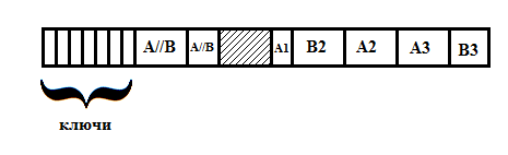
Here A // B is the sorted section, A1 is the underprocessed block, A2, A3, B2 are unprocessed blocks, B3 is an incomplete block at the end (perhaps its real place is before A2 or A3).
In the beginning, we have no merged blocks, T = 0, and the type of ST elements following the buffer is determined by the first key.
To process the next block, we have to write another function SmartMergeLeft (and it is not the last!). At the input, it, like MergeLeft, serves a buffer and two fragments, and the order of these fragments may be incorrect (then when merging it will be necessary in the case of equal elements to take an element from the second fragment). The function should rearrange elements to the beginning only as long as both fragments are non-empty. As soon as one of them ends, it must transfer the remaining elements of the other fragment to the end (if the second fragment ended earlier), report their number, and then in what fragment they were.
Like that:

In the first case, elements from B first ran out, and at the end there were the last elements from A, and in the second - the opposite.
Using this function, we can easily move up one block. If the type of the next block is the same as the last unprocessed elements, we change them with the buffer, and say that T = 0, and the new block is raw (the situation is the same as at the beginning). If the types are different, we call SmartMergeLeft, and she does everything herself - the elements that will remain at the end of the block will be unprocessed.
So, turning over the blocks, we will reach either the end, or to the place where there should be an incomplete block from the end of fragment B. Here we have several options.
Either the last remaining unprocessed elements are from fragment B. Then the last of these elements is smaller than the first element from the next block A (if there is one), and we can safely exchange the raw elements with the buffer.
Either these elements are from fragment A. Then we simply virtually paste them onto the blocks following them (again, if they exist).
In both cases, we get the same situation - the buffer, followed by elements from fragment A, then no more than S elements from fragment B. Ready situation for the MergeLeft function. Call it - and the fragments are merged, and the buffer was after them.
We go through this procedure for all pairs of fragments of length G, until we reach the end of the data array. Then we shift all the data to the right by S elements (returning the buffer to the beginning), and double the value of S.
The end of the cycle.
A.3. Completion.
We have a sorted array of data, before which the keys found at the beginning randomly go. Sort them (again with inserts), and we will only have to merge two sorted fragments without using an additional buffer. This time we will be saved by the fact that one of them is very short.
The function MergeWithoutBuffer receives two sorted fragments of length P and Q as input. Suppose that P <Q. As long as the first element of the first fragment is not larger than the first element of the second fragment, we will decrease P by 1, shifting the beginning of the fragment to the right. If P reaches zero - we won. Otherwise, we will find with the help of BinSearchLeft the correct position k of the first element in the second fragment, and with the help of ROTATE we will change the first fragment and the first k elements of the second fragment. Reduce Q by k, shift the beginning of the fragments. If Q has reached zero, the function is executed, otherwise we repeat it from the beginning. The complexity of this function is P ^ 2 + Q. If initially P≥Q, then we do the same, but in a mirror order.
To complete the sorting call MergeWithoutBuffer (Arr, K + S, NKS). All is ready.
Case B. There are few different keys, but more than three.
In this situation, we do not have space for the buffer and the keys at the same time, we will use them in turn. Let various keys be all M. We denote by K the maximal power of two that does not exceed M, and leave K keys to us (they are at the beginning of the array), let the rest go to the data.
B.1. Stage of classical merge sorting.
This stage does not differ from A.1, but instead of a buffer of length S, we will use an array of keys of length K (this is a power of two). Walking along the array forward and backward, we get sorted fragments of length G = 2 * K.
B.2. Stage block sorting.
Suppose that fragments of length G are already merged with us, and we want to unite them in pairs. Since we have no buffer, we can choose the block size ourselves. The number of keys for marking blocks in our company does not exceed K. Take K 1 = min (K, K 2 ), where K 2 is a power of two, closest to (2 * G * M) 1/3 (recall that M is the number of different keys in the array). The block size will be S = 2 * G / K 1 .
We sort the keys and blocks as in A.2. This buffer is not needed.
Now we need to go through the array and merge the blocks. Let's write the SmartMergeWithoutBuffer function, which is a hybrid of MergeWithoutBuffer and SmartMergeLeft. It assumes that the first fragment is shorter than the second. It works in the same way as MergeWithoutBuffer, but it takes into account that the order of the fragments could be incorrect, but also reports how many elements and from which fragment remained at the end of the array. Calling this function instead of SmartMergeLeft, and the function MergeWithoutBuffer - instead of MergeLeft at the end, we get merged fragments.
It would seem that here we lost - the maximum block length in the worst case (K = 4, G = N / 2) is N / 4, which means that the SmartMergeWithoutBuffer function may require O (N ^ 2) operations. But we are saved by the fact that the number of different keys in the array is small - and it can be shown that the complexity of SmartMergeWithoutBuffer does not exceed P * m + Q, where m is the number of different keys in the first fragment. And since the sum of the number of different keys across all K / 2 blocks of a fragment of length G (take a deep breath and reread - I can’t make it easier) does not exceed K / 2 + M, no more than O (G) will be spent on merging two fragments of length G operations.
B.3. Completion.
This step is not different from A.3.
Case C. There are no more than three different keys.
Here we write the usual merge sort (without recursion, we sort by 2, then by 4 elements, etc.), and to merge the fragments we use MergeWithBuffers. Since there are few different keys in the array, its complexity will be linear with the length of the merged fragments, which means that the total complexity is O (N * log (N)).
Implementation and conclusions.
The implementation turned out to be cumbersome - almost 400 lines in C ++ (in fact, it is written in C - you just need to transfer the variable descriptions to the beginning of the functions). The speed of work varies greatly for cases A and B. The worst situation is when there are a lot of different keys, but a little bit less than necessary to go to case A - in this situation the algorithm runs slower than in case A, about 3 times. However, the estimated complexity of N * log (N) is preserved.
On large arrays (from about 10 million), the algorithm almost always (except for the cases of a very small number of different keys) beats InPlaceStableSort (the one that is behind O (N * log (N) 2 )). But it cannot with std :: stable_sort: there is always a little memory, and in this case, std :: stable_sort quickly switches to the usual MergeSort, and easily and naturally overtakes everyone, including quicksort :). So the implemented algorithm has only theoretical value.
But still, it exists :)
PS The first picture is a slide from the lecture course R.Sedgewick, Algorithms and Data Structures , Princeton University, Spring 2010
UPDATE: Phase B2 can be greatly accelerated. As long as the number G is sufficiently small, it may happen that (K / 2) ^ 2> = 2 * G. In this case, we can divide the set of keys in half, and use half as a clipboard (and the other half as keys), and merge fragments using the faster method from A2. And go to exchanges without a buffer at the very end, when G approaches the size of the array.
The more keys we have, the longer the merge without a buffer works, but the longer we can do without it.
Experiments show that in the worst case, the algorithm requires no more than 1.61 * N * log 2 N comparisons and 2.12 * N * log 2 N exchanges (with N≤1000000, on random data with a predetermined number of different keys).
Source: https://habr.com/ru/post/205290/
All Articles