Optimize image processing in C ++ using SIMD. Median filter

Introduction

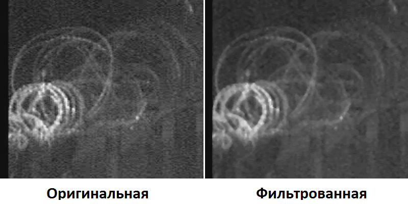
Earlier in the introductory article, I brought up a list of problems that a developer will have to face if he wants to optimize the optimization of image processing using SIMD instructions. Now it's time for a concrete example to show how the above problems can be solved. I thought for a long time which algorithm to choose for the first example, and decided to dwell on median filtering. Median filtering is an effective way to suppress noise that inevitably appears on digital cameras in conditions of low scene illumination. This algorithm is quite resource-intensive - for example, when processing a gray image with a 3x3 median filter, about 50 operations per image point are required. But at the same time, it operates only with 8-bit numbers and it requires relatively little input data to work. These circumstances make the algorithm simple enough for SIMD optimization and at the same time allow you to get a very significant acceleration from it.




For reference, I remind the essence of the algorithm:

• For each point of the original image, a certain neighborhood is taken (in our case, 3x3).
• The points of this neighborhood are sorted by increasing brightness.
• The midpoint (5th for the 3x3 filter) of the sorted neighborhood is recorded in the final image.

For the first example, I decided to simplify the task and consider the case of a gray image (8 bits per pixel) without taking into account boundary effects — for this, the central part of a somewhat larger image was taken for filtering. Of course, in real problems, the boundary points of the image should be calculated using a special algorithm, and sometimes the implementation of these specific algorithms can occupy most of the code, but we will focus on these issues another time. In addition, for similar reasons, it is assumed that the image width is a multiple of 32.
')

Scalar version of the algorithm

1st scalar version

In this initial implementation, the problem was solved head-on: the neighborhood for each point of the original image was copied into an auxiliary array, which was then sorted using the function std :: sort ().

inline void Load(const uint8_t * src, int a[3]) { a[0] = src[-1]; a[1] = src[0]; a[2] = src[1]; } inline void Load(const uint8_t * src, size_t stride, int a[9]) { Load(src - stride, a + 0); Load(src, a + 3); Load(src + stride, a + 6); } inline void Sort(int a[9]) { std::sort(a, a + 9); } void MedianFilter(const uint8_t * src, size_t srcStride, size_t width, size_t height, uint8_t * dst, size_t dstStride) { int a[9]; for(size_t y = 0; y < height; ++y) { for(size_t x = 0; x < width; ++x) { Load(src + x, srcStride, a); Sort(a); dst[x] = (uint8_t)a[4]; } src += srcStride; dst += dstStride; } } 

2nd scalar version

The previous method, however, immediately shows a bottleneck - this is the standard sorting function. It is designed to sort an array of arbitrary size, it has a lot of internal checks, so it will most likely not be the optimal solution for this problem, where the array is small and has a fixed size. In addition, it is not at all necessary for us to sort the array completely; it is enough that in the 4th element we have the value we need. Therefore, we can apply the “network” sorting method (also known as the bitonic sorting method):

 inline void Sort(int & a, int & b) //    { if(a > b) { int t = a; a = b; b = t; } } inline void Sort(int a[9]) //    { Sort(a[1], a[2]); Sort(a[4], a[5]); Sort(a[7], a[8]); Sort(a[0], a[1]); Sort(a[3], a[4]); Sort(a[6], a[7]); Sort(a[1], a[2]); Sort(a[4], a[5]); Sort(a[7], a[8]); Sort(a[0], a[3]); Sort(a[5], a[8]); Sort(a[4], a[7]); Sort(a[3], a[6]); Sort(a[1], a[4]); Sort(a[2], a[5]); Sort(a[4], a[7]); Sort(a[4], a[2]); Sort(a[6], a[4]); Sort(a[4], a[2]); } 

3rd scalar version

Although the first method turned out to be much faster than zero (see the test result below), but it still has one bottleneck - there are a lot of conditional transitions in this method. As you know, modern processors do not like them very much, since they have a pipeline architecture and the possibility of an extraordinary execution of several commands in one clock cycle. Both for the first and for the second conditional transitions are extremely undesirable, since the processor must stop and wait for the results of the calculations in order to find out which branch of the program it should go further. Fortunately, the sorting of two 8-bit values ​​is quite possible to implement without conditional transitions:

 inline void Sort(int & a, int & b) { int d = a - b; int m = ~(d >> 8); b += d&m; a -= d&m; } 

The result of these preliminary scalar code optimizations is the following version of the median filter:

 inline void Load(const uint8_t * src, int a[3]) { a[0] = src[-1]; a[1] = src[0]; a[2] = src[1]; } inline void Load(const uint8_t * src, size_t stride, int a[9]) { Load(src - stride, a + 0); Load(src, a + 3); Load(src + stride, a + 6); } inline void Sort(int & a, int & b) { int d = a - b; int m = ~(d >> 8); b += d&m; a -= d&m; } inline void Sort(int a[9]) //    { Sort(a[1], a[2]); Sort(a[4], a[5]); Sort(a[7], a[8]); Sort(a[0], a[1]); Sort(a[3], a[4]); Sort(a[6], a[7]); Sort(a[1], a[2]); Sort(a[4], a[5]); Sort(a[7], a[8]); Sort(a[0], a[3]); Sort(a[5], a[8]); Sort(a[4], a[7]); Sort(a[3], a[6]); Sort(a[1], a[4]); Sort(a[2], a[5]); Sort(a[4], a[7]); Sort(a[4], a[2]); Sort(a[6], a[4]); Sort(a[4], a[2]); } void MedianFilter(const uint8_t * src, size_t srcStride, size_t width, size_t height, uint8_t * dst, size_t dstStride) { int a[9]; for(size_t y = 0; y < height; ++y) { for(size_t x = 0; x < width; ++x) { Load(src + x, srcStride, a); Sort(a); dst[x] = (uint8_t)a[4]; } src += srcStride; dst += dstStride; } } 

This version is already significantly (about 5-6 times) ahead of our initial version of the algorithm in speed. And it is based on it that we will implement the SIMD algorithm optimization, as well as carry out a comparison of the speed of the scalar and vector versions of the algorithm.

SIMD version of the algorithm

To illustrate the optimization of the median filtering algorithm using SIMD, I use two sets of instructions SSE2 and AVX2, missing the MMX extension, which is currently outdated and has more historical interest. Fortunately, in order to use SIMD instructions, it is not necessary to use the assembler . Most modern C ++ compilers have intrinsics support (built-in functions with which you can use various processor extensions). Programming using intrinsics is practically the same as programming in pure C. Intrinsic functions are converted by the compiler directly into processor instructions, although working directly with processor registers remains hidden from the programmer. In most cases, a program using intrinsics is not inferior in speed to a program written in assembler.

SSE2 version

The SSE2 integer commands are defined in the <emmintrin.h> header file. The basic type is __m128i - 128 bit vector, which, depending on the context, can be interpreted as a set of 2 64 bit, 4 32 bit, 8 x 16 bit, 16 x 8 bit signed or unsigned numbers. As you can see, they support not only vector arithmetic operations, but also vector logic operations, as well as vector data loading and unloading operations. Below is the optimization of the median filter using SSE2 instructions. The code, I think, is pretty intuitive.

 #include < emmintrin.h > inline void Load(const uint8_t * src, __m128i a[3]) { a[0] = _mm_loadu_si128((__m128i*)(src - 1)); // 128      16    a[1] = _mm_loadu_si128((__m128i*)(src)); a[2] = _mm_loadu_si128((__m128i*)(src + 1)); } inline void Load(const uint8_t * src, size_t stride, __m128i a[9]) { Load(src - stride, a + 0); Load(src, a + 3); Load(src + stride, a + 6); } inline void Sort(__m128i& a, __m128i& b) { __m128i t = a; a = _mm_min_epu8(t, b); //  2- 8       16   b = _mm_max_epu8(t, b); //  2- 8       16   } inline void Sort(__m128i a[9]) //    { Sort(a[1], a[2]); Sort(a[4], a[5]); Sort(a[7], a[8]); Sort(a[0], a[1]); Sort(a[3], a[4]); Sort(a[6], a[7]); Sort(a[1], a[2]); Sort(a[4], a[5]); Sort(a[7], a[8]); Sort(a[0], a[3]); Sort(a[5], a[8]); Sort(a[4], a[7]); Sort(a[3], a[6]); Sort(a[1], a[4]); Sort(a[2], a[5]); Sort(a[4], a[7]); Sort(a[4], a[2]); Sort(a[6], a[4]); Sort(a[4], a[2]); } void MedianFilter(const uint8_t * src, size_t srcStride, size_t width, size_t height, uint8_t * dst, size_t dstStride) { __m128i a[9]; for(size_t y = 0; y < height; ++y) { for(size_t x = 0; x < width; x += sizeof(__m128i)) { Load(src + x, srcStride, a); Sort(a); _mm_storeu_si128((__m128i*)(dst + x), a[4]); // 128      16    } src += srcStride; dst += dstStride; } } 

AVX2 version

The AVX2 integer commands are defined in the <immintrin.h> header file. The base type is __m256i - 256 bit vector, which, depending on the context, can be interpreted as a set of 4 64 bit, 8 32 bit, 16 16 bit, 32 8 bit signed or unsigned numbers. Although the AVX2 instruction set largely repeats the SSE2 instruction set (taking into account the doubled width of the vector), but it also contains quite a lot of instructions that have no analogues in SSE2. Below is the optimization of the median filter using AVX2 instructions.

 #include < immintrin.h > inline void Load(const uint8_t * src, __m256i a[3]) { a[0] = _mm256_loadu_si256((__m128i*)(src - 1)); // 256      32    a[1] = _mm256_loadu_si256((__m128i*)(src)); a[2] = _mm256_loadu_si256((__m128i*)(src + 1)); } inline void Load(const uint8_t * src, size_t stride, __m256i a[9]) { Load(src - stride, a + 0); Load(src, a + 3); Load(src + stride, a + 6); } inline void Sort(__m256i& a, __m256i& b) { __m256i t = a; a = _mm256_min_epu8(t, b); //  2- 8       32   b = _mm256_max_epu8(t, b); //  2- 8       32   } inline void Sort(__m256i a[9]) //    { Sort(a[1], a[2]); Sort(a[4], a[5]); Sort(a[7], a[8]); Sort(a[0], a[1]); Sort(a[3], a[4]); Sort(a[6], a[7]); Sort(a[1], a[2]); Sort(a[4], a[5]); Sort(a[7], a[8]); Sort(a[0], a[3]); Sort(a[5], a[8]); Sort(a[4], a[7]); Sort(a[3], a[6]); Sort(a[1], a[4]); Sort(a[2], a[5]); Sort(a[4], a[7]); Sort(a[4], a[2]); Sort(a[6], a[4]); Sort(a[4], a[2]); } void MedianFilter(const uint8_t * src, size_t srcStride, size_t width, size_t height, uint8_t * dst, size_t dstStride) { __m256i a[9]; for(size_t y = 0; y < height; ++y) { for(size_t x = 0; x < width; x += sizeof(__m256i)) { Load(src + x, srcStride, a); Sort(a); _mm256_storeu_si256((__m256i*)(dst + x), a[4]); // 256      32    } src += srcStride; dst += dstStride; } } 

Note: To get maximum acceleration from optimization, the code that contains AVX2 instructions should be compiled with the following compiler option: (/ arch: AVX for Visual Studio 2012, -march = core-avx2 for GCC). In addition, it is very desirable that the code does not include the alternation of AVX2 and SSE2 instructions, since switching the operating mode of the processor in this case will adversely affect the overall performance. Based on the above, it is advisable to have the AVX2 and SSE2 versions of the algorithms in different ".cpp" files.

Testing

Testing was performed on gray images of 2 MB (1920 x 1080). To improve the accuracy of measuring time, the tests were run several times. The execution time was obtained by dividing the total test execution time by the number of runs. The number of runs was chosen in such a way that the total execution time was not less than 1 second, which should provide two signs of accuracy when measuring the execution time of the algorithms. The algorithms were compiled with maximum optimization for 64 bit Windows 7 on Microsoft Visual Studio 2012 and run on an iCore-7 4770 processor (3.4 GHz).

Execution time, ms			Relative acceleration
Best scalar	SSE2	AVX2	Best scalar / SSE2	Best Scalar / AVX2	SSE2 / AVX2
24.814	0.565	0.424	43.920	58.566	1.333

Conclusion

As can be seen from the result of the tests, the acceleration of the median filtering algorithm from using SIMD instructions on modern processors can reach from 40 to 60 times. As it seems to me, this is a sufficient value to bother with optimization (if, of course, execution speed is important in your program). In this publication I tried to simplify the code used as much as possible.
So beyond the framework there were issues related to the alignment of data, with the processing of boundary points, and much more.
I will try to reveal these questions in the following articles. If the reader is interested in how the combat code that implements this functionality will look like, then he will be able to find it here .