Gnuplot vs. 2MASS

This article focuses on the benefits of low-level computing using the example of the atlas of stellar objects 2MASS .
2MASS is ~ 471 million objects for which coordinates are given, as well as accompanying information, a total of 60 attributes.
Physically - this is 50GB of source gzipnutyh text files.
Is it possible to work with such a base without resorting to "heavy artillery"?
Let's try.

Prelude

This work was carried out in 2009 and was part of the efforts of DataEast to create its own geo-DBMS.
The goal was to debug, profile and make benchmark query processor.
As a query language, the dialect Turorial D was chosen, or rather its part relating to relational algebra. The dialect was adapted to the requirements of real life, in particular, added the ability to work with cursors.

However, this is just a context and the purpose of this post is not a story about past victories that “melted away like tears in the rain”, but a demonstration of the technique of maximum transfer of calculations directly to the DBMS cursor.
Of course, this technique can also be applied by means of PL / SQL using stored procedures and / or using aggregates.

Introduction

It makes no sense to dwell on the process of preparing the data, let's just say that it took 8 hours and 26 minutes to fill the data and 1 hour and 17 minutes to spatial indexing.
Complete with the initial data there is a verification request.

select count(*) as rows, sum(pts_key::bigint) as sum_pts_key, sum(pxcntr::bigint) as sum_pxcntr, sum(scan_key::bigint) as sum_scan_key, sum(scan::bigint) as sum_scan, sum(ext_key::bigint) as sum_ext_key, sum(coadd_key::bigint) as sum_coadd_key, sum(coadd::bigint) as sum_coadd, sum(mp_flg) as sum_mp_flg, sum(gal_contam) as sum_gal_contam, sum(use_src) as sum_use_src, sum(dup_src) as sum_dup_src, sum(nopt_mchs) as sum_nopt_mchs, sum(phi_opt::bigint) as sum_phi_opt, sum(dist_edge_ew::bigint) as sum_dist_edge_ew, sum(dist_edge_ns::bigint) as sum_dist_edge_ns, sum(err_ang::bigint) as sum_err_ang FROM twomass_psc; 

In our case, this query will look like

 select "PSC" chew { "rows" INTEGER, "sum_pts_key" INTEGER, "sum_pxcntr" INTEGER, "sum_scan_key" INTEGER, "sum_scan" INTEGER, "sum_ext_key" INTEGER, "sum_coadd_key" INTEGER, "sum_coadd" INTEGER, "sum_mp_flg" INTEGER, "sum_gal_contam" INTEGER, "sum_use_src" INTEGER, "sum_dup_src "INTEGER, "sum_nopt_mchs" INTEGER, "sum_phi_opt" INTEGER, "sum_dist_edge_ew" INTEGER, "sum_dist_edge_ns" INTEGER, "sum_err_ang" INTEGER } hook "init" { "rows" := 0; "sum_pts_key" := 0; ... "sum_err_ang" := 0; } hook "row" { "rows" := "rows" + 1; if (not isnull("pts_key/cntr")) then "sum_pts_key" := "sum_pts_key" + "pts_key/cntr"; end if; ... if (not isnull("err_ang")) then "sum_err_ang" := "sum_err_ang" + "err_ang"; end if; } hook "finit" { call __interrupt (); }; 

The result of the execution is:

 INFO: start [04/Jun/2009:09:37:45:822] ----------------------------------------------------------------- rows sum_pts_key sum_pxcntr sum_scan_key sum_scan sum_ext_key sum_coadd_key sum_coadd sum_mp_flg sum_gal_contam sum_use_src sum_dup_src sum_nopt_mchs sum_phi_opt sum_dist_edge_ew sum_dist_edge_ns sum_err_ang ----------------------------------------------------------------- 470992970 306810325437475788 306815556538478936 16902776758555 32666066948 2048692118201 388758631396659 64617139213 16048 729878 464456155 79798372 369187043 64916239773 69388217174 2670725813652 29279563815 ----------------------------------------------------------------- INFO: stop [04/Jun/2009:12:35:59:571] 

Here, the chew operator is used to convert the original data stream (the entire table) to synthetic with certain fields that become local variables. The hook statement is used (similar to SQL aggregates) for subscribing to events — the start / stop of a stream and the receipt of a string. When __interrupt is called , the current values ​​of local variables fall into the resultset.
')
The results coincide with the verification, so the data is prepared for work.
Opening hours - 3 hours, about 10 minutes per column for continuous viewing. This speed (on Intel Core2 P4-2.4 GHz, 2Gb, disk ST3400620AS) is typical for all further requests. On the other hand, if we unpacked the source text files and processed them through GAWK, for example, it would take 50GB of 50 MB / s = 1000 seconds to read the data and the same amount to unpack, 35 minutes only to organize the stream. It took an hour and a half to decompress and run all the data through wc.

For those who want to see everything with their own eyes, there is a piece of the sky with a defect plate:

Some people take him for the battle orders of the imperial fleet.

Data mining

Simple statistics. Max, Min, Avg - let's play with the column “jm” (Default J-band magnitude).

 select "PSC" chew { "nrows" INTEGER, "nulls_j_m" INTEGER, "num_j_m" INTEGER, "sum_j_m" RATIONAL, "avg_j_m" RATIONAL, "max_j_m" RATIONAL, "min_j_m" RATIONAL } hook "init" { "nrows" := 0; "nulls_j_m" := 0; "num_j_m" := 0; "sum_j_m" := 0; "avg_j_m" := 0; "max_j_m" := -1e66; "min_j_m" := 1e66; } hook "row" { nrows := nrows + 1; if (isnull("j_m")) then "nulls_j_m" := "nulls_j_m" + 1; else "num_j_m" := "num_j_m" + 1; "sum_j_m" := "sum_j_m" + "j_m"; if ("max_j_m"<"j_m") then "max_j_m" := "j_m"; end if; if ("min_j_m">"j_m") then "min_j_m" := "j_m"; end if; end if; } hook "finit" { "avg_j_m" := "sum_j_m" / "num_j_m"; call __interrupt (); }; 

Result:

 INFO: start [04/Jun/2009:15:00:54:821] -------------------------------------------------------------------- nrows nulls_j_m num_j_m sum_j_m avg_j_m max_j_m min_j_m -------------------------------------------------------------------- 470992970 19 470992951 7.15875e+009 15.1993 25.86 -2.989 -------------------------------------------------------------------- INFO: stop [04/Jun/2009:15:18:47:743] 

Dispersion:

 select "PSC" chew { "nrows" INTEGER, "nulls_j_m" INTEGER, "num_j_m" INTEGER, "disp_j_m" RATIONAL } hook "init" { "nrows" := 0; "nulls_j_m" := 0; "num_j_m" := 0; "disp_j_m" := 0; var tmp rational; var tavg rational; tavg := 15.1993; -- previously calculated } hook "row" { nrows := nrows + 1; if (isnull("j_m")) then "nulls_j_m" := "nulls_j_m" + 1; else "num_j_m" := "num_j_m" + 1; tmp := "j_m" - tavg; tmp := tmp * tmp; "disp_j_m" := "disp_j_m" + tmp; end if; } hook "finit" { "disp_j_m" := "disp_j_m" / "num_j_m"; call __interrupt (); }; 

Result :

 INFO: start [04/Jun/2009:15:48:27:274] -------------------------------------------------------------------- nrows nulls_j_m num_j_m disp_j_m -------------------------------------------------------------------- 470992970 19 470992951 1.98223 -------------------------------------------------------------------- INFO: stop [04/Jun/2009:16:05:01:946 

Bar chart:

 select "PSC" chew { "j_m_cell" rational, "num" INTEGER } hook "init" { var tmp integer; var tmp2 integer; var tmax rational; tmax := 26.; -- previously calculated var tmin rational; tmin := -5.; -- previously calculated var ncells integer; ncells := 500; var tcell rational; tcell := (tmax - tmin)/ncells; var htptr integer; htptr := hti_alloc (0); call hti_set (htptr, 0, 0); } hook "row" { if (not isnull("j_m")) then tmp := ("j_m" - tmin)/tcell; tmp2 := hti_get (htptr, tmp); tmp2 := tmp2 + 1; call hti_set (htptr, tmp, tmp2); end if; } hook "finit" { tmp := 0; while tmp < ncells; begin; "j_m_cell" := tmin + tcell * tmp + tcell * 0.5; "num" := hti_get (htptr, tmp); tmp := tmp + 1; call __interrupt (); end; end while; call hti_free (htptr); }; 

Histogram cells are accumulated using a hash table due to the absence of arrays in the language. In this case, the result will be a printout of the cells of the histogram, which is convenient to look through gnuplot . In the picture below, printouts are also added in columns “km” (Default Ks-band magnitude) and “hm” (Default H-band magnitude).


3D
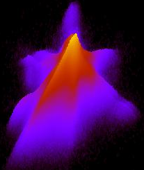
Well, the “km” and “hm” on the histogram look very similar, but what about the joint distribution?

 select "PSC" chew { "cell" rational, "num" INTEGER } hook "init" { var tmp integer; var tmp2 integer; var tmp4 integer; var tmax rational; tmax := 25; var tmin rational; tmin := -5.; var ncells integer; ncells := 512; var tcell rational; tcell := (tmax - tmin)/ncells; var "hnd" integer; hnd:= img_create ( ncells, ncells, tmin, tmin, tmax, tmax, 1); var cl integer; cl := img_alloc_color (hnd, 255,0,0); } hook "row" { if ((not isnull("h_m")) and (not isnull("k_m"))) then tmp := img_get_point (hnd, "h_m", "k_m"); tmp := tmp + 1; call img_draw_point (hnd, "h_m", "k_m", tmp); end if; } hook "finit" { tmp := 0; while tmp < ncells; begin; tmp2 := 0; while tmp2 < ncells; begin; tmp4 := img_get_point (hnd, tmin + tcell * tmp, tmin + tcell * tmp2); call print ((tmin + tmp * tcell)+' '+ (tmin + tmp2* tcell)+' '+tmp4+'\n'); if tmp4 > 0 then tmp4 := cl; else tmp4 := 0; end if; call img_draw_point (hnd, tmin + tcell * tmp, tmin + tcell * tmp2, cl); tmp2 := tmp2 + 1; end; end while; tmp := tmp + 1; end; end while; call img_saveas (hnd, 'stat4.gif'); call img_destroy (hnd); }; 

In this example, to store a two-dimensional histogram, the image of the image obtained by means of the GD plug-in was used, and the logarithms of hits in the cells are viewed again using gnuplot mode in pm3d mode.

Similar picture for the distribution of “j_m“ - “k_m“ against “h_m“ - “k_m“:

The construction of these histograms takes ~ 35 min - 12 min per column.
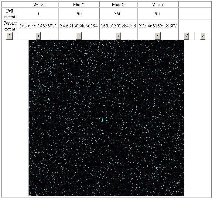
But what if we need to build such a distribution over a specific spatial area? Can we do it in seconds? Of course:
Sampling with spatial constraints .

 select "PSC" where sp_overlap ("Point", [rational:xmin], [rational:ymin], [rational:xmax], [rational:ymax]) chew { "m_cell" rational, "num" INTEGER } … -- below is the same text 

Adding sp_overlap changed the source identifier flow from the table to the spatial index.

In the lower left corners of the cells are the extents of the samples.

What about attribute restrictions ?
It is as easy as limiting in space.

 select "PSC" where “j_snr” < 10. -- or you may combine your restrictions adding -- and sp_overlap ("Point", … ) chew { "m_cell" rational, "num" INTEGER } … -- below is the same text 

And here is the result.

Total

What gives us the transfer of calculations to the cursor?

• speed , processing the read data on the spot, we are free to serialize, send over the network, receive, deserialize ...
• saved resources , for example, half a billion lines, being sent over the network, will permanently occupy a fair share of its bandwidth

And how do we face such a technique?

• You have to do everything yourself, and this is a potential source of errors.
• Algorithms in which really a lot of calculations are not very convenient to perform on a common server.
• Not all calculations can be done in the stream.

This is all true, but the author does not argue that it is always necessary to do this, this is just one of many tools for working with data, albeit convenient, especially for the research part of the work, for example, when it is necessary to quickly check and modify hypotheses.