A critical look at the Lorenz attractor

1. About the Lorenz attractor

Edward Norton Lorenz (1917 - 2008) is the founder of chaos theory, which is very popular in science today. He attended Dartmouth College, New Hampshire, USA, and Harvard University, Cambridge. During World War II, he served as a meteorologist at the US Army Air Corps, then until the end of his days he worked as a professor at the Massachusetts Institute of Technology.

In 1963, his article “Deterministic Nonperiodic Flow” was published in the Journal of the Atmospheric Sciences (Russian translation: Lorenz E. Deterministic non-periodic flow // Strange attractors. - Moscow: Mir, 1981, pp. 88-117), which laid not only the foundations of the theory of chaos, but also changed the concept of modeling weather phenomena. In this work, for the first time, a nonlinear autonomous system of ordinary third-order differential equations (dynamic system) was obtained from the system of Navier-Stokes equations, describing the movement of air flows in a flat liquid layer of constant thickness when decomposing the flow velocity and temperature into double Fourier series with subsequent truncation - the second harmonics:
')
(one)

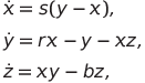
where s , r and b are some positive numbers, system parameters. Usually, studies of the Lorentz system are carried out at s = 10 , r = 28 and b = 8/3 (classical values ​​of the parameters).

In general, chaos theory is a branch of mathematics that studies the behavior of deterministic dynamical systems, where solutions have a rather complicated structure, so it seems that they behave randomly in time. The deterministic system is a system, equations of motion, parameters and initial conditions of which are known and are not random (Moon F. Chaotic oscillations. - M .: Mir, 1990).

Dynamic system (1) also occurs in other processes:

1. Convection in a toroidal tube (Landa PS Nonlinear oscillations and waves. - M: LIBROCOM, 2010, p. 454-455);
2. Single-mode laser (LA Pokrov. Solution of the system of Lorentz equations in the asymptotic limit of a large Rayleigh number. I. The Lorentz system in the simplest laser quantum model and the averaging method applied to it // Theoretical and Mathematical Physics, 1985, vol. 62, No. 2, pp. 272-290);
3. Oscillator with inertial excitation (Neimark, Yu.I., Landa, PS, Stochastic and Chaotic Oscillations. - M: LIBROCOM, 2009, pp. 288-295).

For any solution of the Lorentz system, there exists a moment in time when the corresponding phase trajectory plunges forever into a sphere of a fixed radius. Therefore, there exists a limit set — the Lorentz attractor — to which all trajectories of a dynamical system attract (Nemytsky V.V., Stepanov V.V. Qualitative Theory of Differential Equations. - M .: Editorial URSS, 2004, p. 357-359). Thus, the attractor determines the behavior of the solutions of system (1) over large periods of time.

Due to the lack of accurate methods for solving general nonlinear dynamic systems, numerical methods are often used to analyze the structure of an attractor, such as, for example, combining an explicit Euler scheme with a central difference scheme, Adams, using higher derivatives, and Runge-Kutta 4th order In the case of classical values ​​of system parameters, instability of its solutions is observed, since the equilibrium positions of the system are of saddle type. This limits the use of these methods, since the total error increases with an increase in the integration interval. Thus, small changes in the initial conditions of the system (1) (ie, the atmosphere) can lead to significant consequences over time.

In the 70s. On the basis of the results of numerical experiments, Hookenheimer, Williams and York formulated a hypothesis about the structure of the Lorenz attractor with the classical values ​​of the system parameters, however, this hypothesis was not rigorously proved. In 2000, Steven Smale compiled a list of 18 of the most significant mathematical problems of the 21st century. The problem of the structure of the attractor Lorenz was included in this list at number 14. It is believed that it was solved by Warwick Tucker in 2002 using interval arithmetic, but many mathematicians did not accept his proof, if only because the presence of periodic solutions in system (1).

In the literature devoted to the numerical study of the Lorentz system with the classical values ​​of its parameters, conclusions about the structure of the attractor are often made on the basis of data obtained from a computational experiment (for example, that the attractor contains cycles). At the same time, there are no sufficient justifications for choosing a step, with which types of real numbers one had to work, and at what length of time calculations were made.


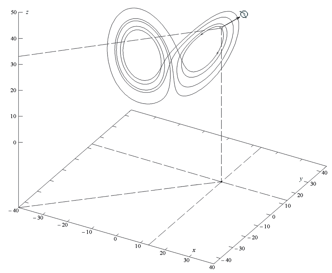
Fig. 1. An arc of a trajectory constructed on the time interval [0; 6.827] for x (0) = 13.41265629, y (0) = 13.46430003, z (0) = 33.46156416.

By the Birkhoff theorem (Nemytsky VV, Stepanov VV The qualitative theory of differential equations. - M .: Editorial URSS, 2004, p. 402) the Lorenz attractor contains recurrent trajectories, and each recurrent motion is stable along Poisson. This means that there will be arbitrarily large values ​​of the moments of time that the point of the trajectory of the system is in any neighborhood of its initial position. Such a recurrent motion can also be a cycle, but it is impossible to draw a conclusion about this, based on the trajectory return found in some neighborhood of the initial conditions. As shown by calculations (Fig. 1), in the Lorenz system, the dynamics of the behavior of solutions on an attractor is quite complex — the recurrent trajectories contained in it can, for example, be described by almost periodic solutions or have a more complex structure. I have built an example of a non-autonomous system with this behavior of solutions.

2. Modeling the dynamics of the Lorentz system

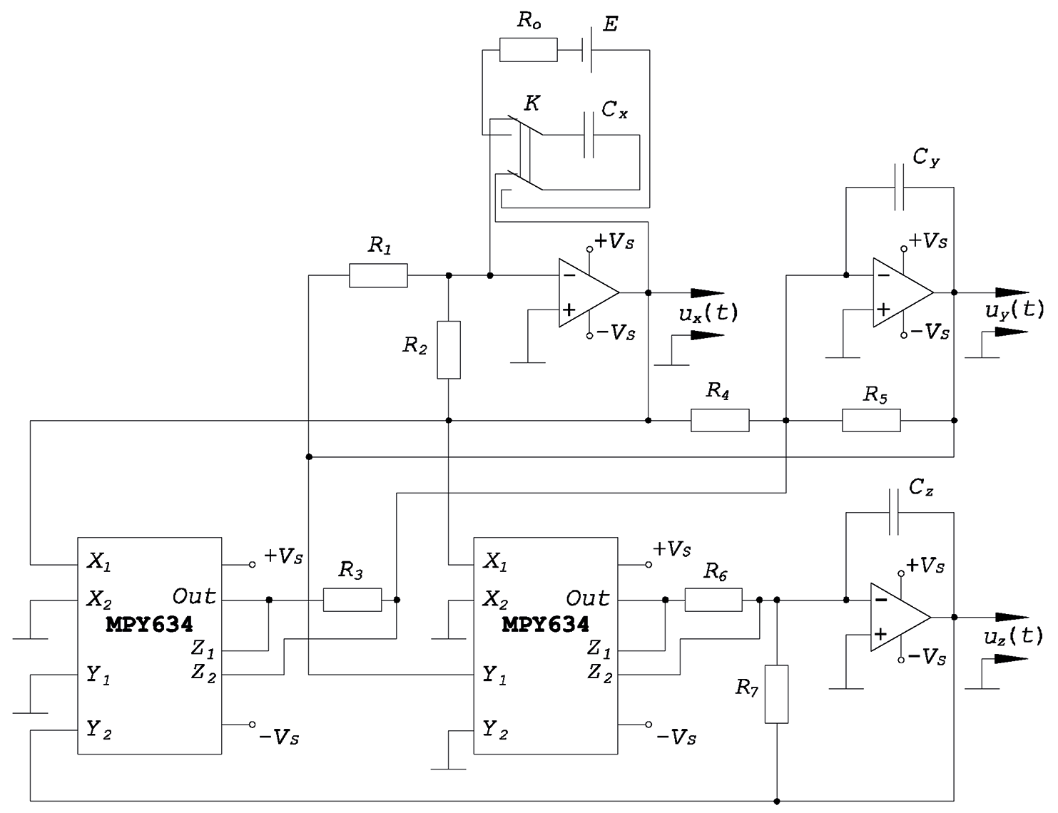
Fig. 2. Scheme of the oscillation generator describing the dynamics of the Lorentz system.

For generating signals (chaotic oscillations) describing trajectories on attractors of dynamic systems with certain types of non-linearities of the right-hand parts, physical modeling using electrical circuits / or analog computers / is also used in practice (Dmitriev AS, Panas AI chaos: new media for communication systems. - M .: Fizmatlit, 2002).

Consider the electrical circuit of the oscillator, shown in Fig. 2, as an alternative to numerical modeling. Since the Lorenz system is of the third order, then three integrators based on operational amplifiers are needed to create the dynamics of voltage variation in the circuit, since noise problems are associated with differentiators. In this case, for constructing the circuit and recording the integral equations, we used the basic switching circuit of the modern analog multiplier MPY634 , shown in fig. 3 in the official documentation of the manufacturer of the chip. We have:



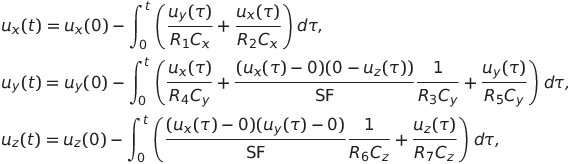
Where , and - instantaneous values ​​of voltages corresponding to the functions x ( t ) , y ( t ) and z ( t ) (a pair of these voltages can be applied to the oscilloscope plates - the resulting complex figure is a projection of the trajectory of the Lorentz system onto the corresponding plane), and 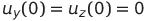- initial voltages on capacitors , and accordingly, SF = 10 V is the scale factor of the multiplier.

The capacitor is initially charged. from power supply E ; resistor provided for recharging (the state of the key K is shown in the figure in the generator circuit). The remaining capacitors have zero initial charge. In fact, we set the initial conditions for the system (1). The initial charging circuit can be changed (for example, to charge two capacitors), except for the situation when 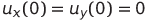. This is explained by , and Is a particular solution of the system (1), where - arbitrary constant. It is clear that in this case there will be no fluctuations.

Make a replacement and differentiate by time both sides of each integral equation. Will get

(2)

We will model the dynamics at the classical values ​​of the parameters of the system (1). We set the values ​​of resistances and capacities equal



Then system (2) takes the form

(3)

Making a (3) replacement



get the Lorentz system. Insofar as



then from the introduced replacement it follows that the absolute value of the voltage will not exceed the value of 7.44 V , which is provided for by the documentation of the multiplier MPY634 . The value of E can be chosen equal to 1.5 V (emf of a finger battery).

The accuracy of the presented model is determined by the errors of real capacities and resistances, as well as the frequency characteristics of integrators and multipliers.

PS

Recently, I made a report on this topic at a mathematical conference. You can watch it here (I apologize in advance for the quality of the video). There you can also download the report materials (it is better to view the presentation synchronously with the report, because of the quality of the video, it is not clearly visible).