Monte Carlo simulation of the blogosphere
As an epigraph:
I was interested in the question: how exactly does the growth of popularity of talented "poets", which everyone starts to read in a situation where everyone is both a "poet" and a reader, is happening. I put the word “poet” in quotes because in reality everything described in the epigraph resembles the current blogosphere and social networks.
In this post there will be a lot of formulas, graphs and any near-science boltology. I will show an example of modeling a small social network using JavaScript using Monte-Carlo methods. I do not pretend to the ultimate truth. However, it is likely that this post will be useful for those who want to do something similar.
')
So, to begin with, let's write out the features of our highly simplified virtual “blogosphere”.
1. There are N participants, each of them is characterized by the number i = 1 ... N.
2. Each of them reads K pieces of other participants (friends). All this is defined by a two-dimensional array:
P i, k contains the number of the k- th friend of the i- th participant.
3. For each participant, Hat’s pieces (for all equally) “enemies” are randomly selected - the numbers of those participants whom this participant never zafrendit himself.
4. Each participant i has a personal property - a measure of talent. Stored in array T i .
5. The value of T i is randomly distributed to each participant at the very beginning.
6. Also at the beginning, each participant receives K random friends.
7. At the same time, the number of readers of each R i is already random, at least roughly close to the value of K (if everyone reads K random people, then he himself will be read about as many).
8. Sets the number of Days of the experiment.
9. Positive numbers q and r : q characterize how important the quality of posts is for participants, and r characterizes how important the existing popularity is when making the decision on frending.
By day, I mean one iteration of the main loop. What happens in this cycle.
1. Each i participant writes 1 post quality Q i . The value of Q i is a random variable, however, its distribution depends on the talent T i . The higher the value of T i , the more likely it is to see from the participant i posts with high quality Q i .
2. For each participant i , one friend is selected, the quality of the last three posts of which is lower than that of the other friends. We will replace this friend with a new one.
3. We are looking for a replacement candidate among friends of friends, sifting out those who are already friends or enemies among them.
4. To each of the list of applicants for a replacement, we assign a number characterizing the probability with which we choose it. This probability depends on the quality of his last three posts Q i and the already popular popularity of R i . The probability in my model is described by a simple formula:

As you can see, the better the posts of the candidate and the more popular he is, the more likely he will be to choose him. The constant C , the same for all applicants, is used for normalization, so that the sum of all probabilities for all candidates is equal to one.
5. Randomly, but taking into account not equal probabilities, we select a replacement from the prepared list and replace the old friend with a new one. And so we do with each of the N.
The main indicator that is interesting in this study is the number of readers R i , how it changes every day. Specifically - the first three participants with the greatest talent.
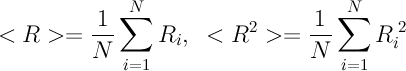
6. After all the replacements, we calculate the variance value D of the distribution R i . The number D characterizes the standard deviation from the average number of readers. For example, if each of N has the same number of readers, then the average is exactly the same number, and deviations from the average are not (all are the same!), Then the variance is zero. But the greater the inequality in the number of readers, the greater will be the variance of D. Here is the expression for her:

where the angle brackets denote averaging over all participants:
7. The required statistics are written to the arrays for further output to the graphs and the cycle repeats again until the Days of Days have passed.
Also in the framework of the simulation is carried out such an experiment. One of the ordinary participants (Rabbit) on the day of DayX suddenly magically receives a talent of the same magnitude as the most talented participant + one reader. How will he climb to the top of his fame, considering that by the time of DayX the talents have probably already received their maximum of readers? Its success is also being monitored.
Delving into the details. One of the tasks of the Monte Carlo methods is to generate random numbers with a given distribution.
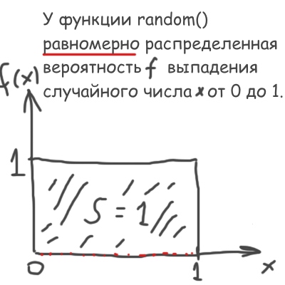
That is, from the standard machine function random () with a uniform distribution (picture above) you need to make your own, special:
Recall that the value of f (x) dx is, by definition, equal to the probability of a number falling between x and x + dx . Therefore, of course, the integral of f (x) should be equal to 1.
For some special types of f (x), the problem is solved analytically. So, to generate random talent T, I used the decaying exponent:
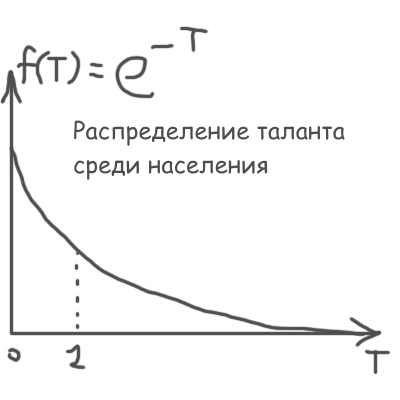
I used exactly the same exponent to further generate random quality Q posts of a participant with a given talent T :

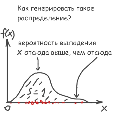
So, how to generate Q distributed according to the law f (x) , which is shown in the figure above, using the random number Rnd evenly distributed from 0 to 1? Very simple:
 .
.
Now, about what can be the maximum variance and why the "enemies" are introduced.
In the first version, without antipathy, the situation developed simply: the list of K friends for all N participants was the same and contained the first K most talented. Well, K + 1 also had readers at the expense of those K first. This situation corresponds to the maximum value of the variance D , which is approximately equal (assuming 1 << K << N):
 .
.
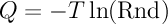
The more “enemies” we enter, the smaller the resulting variance. So, here are the simulation results:
In case people value popularity more than the quality of posts:
In most cases, the set of popularity is slow. Temporary failures of popularity are observed (here is a possible answer to those who regularly create posts in LiveJournal that here are bastards, again social capital (SC) was cut down!). This is due to the peculiarity of the chosen distribution function, when, for any talent, most posts tend to be close to zero.
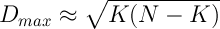
The case if people equally appreciate the popularity and quality of posts:
It should be noted that different implementations of the algorithm with the same parameters can lead to very diverse dependencies of the number of readers on time. There are similarities, but very vague. However, the dependence of the dispersion, as an integral, averaged value, is almost unchanged with the same parameters. Two parameters are important depending on the dispersion on time: the time for reaching the asymptotics, that is, the time during which the blogosphere comes to an equilibrium state, after which mass overflows of readers cease to occur, and also the asymptotics itself, which is determined by the ratio between N and Hat .
The algorithm was implemented in JavaScript, the graphics were drawn using the Google API Chart, so that any user of a modern computer can easily reproduce these results, or even improve their implementation.
A small pleasant (because easy) question for the future: how accurately will it be to count the variance of the distribution R i , if we average not over the entire set of N , but by the smaller number n << N randomly selected participants? After all, if it turns out that a small random sample displays the entire population of bloggers well, then you can, for example, monitor the “weather” in the same LiveJournal - calculating the variance every day and evaluating its trends.
- They have a lot of poets there. Everyone writes poetry, and every poet,
naturally wants to have a reader. The reader is a creature
unorganized, he does not understand this simple thing. He is pleased
reads good poems and even memorizes them, and bad ones know not
wishes It creates a situation of injustice, inequality, and since
the people there are very delicate and eager for everyone to be well established
special profession - reader. Some of them specialize in iambus, others - in chorea, and Konstantin Konstantinovich - a major specialist in amphibrachia and
masters the Alexandrian verse now, acquires a second specialty.
This workshop is naturally harmful, and readers are not only relied upon.
food, but also frequent short-term vacation.
Strugatsky, the Tale of the Troika
I was interested in the question: how exactly does the growth of popularity of talented "poets", which everyone starts to read in a situation where everyone is both a "poet" and a reader, is happening. I put the word “poet” in quotes because in reality everything described in the epigraph resembles the current blogosphere and social networks.
In this post there will be a lot of formulas, graphs and any near-science boltology. I will show an example of modeling a small social network using JavaScript using Monte-Carlo methods. I do not pretend to the ultimate truth. However, it is likely that this post will be useful for those who want to do something similar.
')
So, to begin with, let's write out the features of our highly simplified virtual “blogosphere”.
1. There are N participants, each of them is characterized by the number i = 1 ... N.
2. Each of them reads K pieces of other participants (friends). All this is defined by a two-dimensional array:
P i, k contains the number of the k- th friend of the i- th participant.
3. For each participant, Hat’s pieces (for all equally) “enemies” are randomly selected - the numbers of those participants whom this participant never zafrendit himself.
4. Each participant i has a personal property - a measure of talent. Stored in array T i .
5. The value of T i is randomly distributed to each participant at the very beginning.
6. Also at the beginning, each participant receives K random friends.
7. At the same time, the number of readers of each R i is already random, at least roughly close to the value of K (if everyone reads K random people, then he himself will be read about as many).
8. Sets the number of Days of the experiment.
9. Positive numbers q and r : q characterize how important the quality of posts is for participants, and r characterizes how important the existing popularity is when making the decision on frending.
By day, I mean one iteration of the main loop. What happens in this cycle.
1. Each i participant writes 1 post quality Q i . The value of Q i is a random variable, however, its distribution depends on the talent T i . The higher the value of T i , the more likely it is to see from the participant i posts with high quality Q i .
2. For each participant i , one friend is selected, the quality of the last three posts of which is lower than that of the other friends. We will replace this friend with a new one.
3. We are looking for a replacement candidate among friends of friends, sifting out those who are already friends or enemies among them.
4. To each of the list of applicants for a replacement, we assign a number characterizing the probability with which we choose it. This probability depends on the quality of his last three posts Q i and the already popular popularity of R i . The probability in my model is described by a simple formula:
As you can see, the better the posts of the candidate and the more popular he is, the more likely he will be to choose him. The constant C , the same for all applicants, is used for normalization, so that the sum of all probabilities for all candidates is equal to one.
5. Randomly, but taking into account not equal probabilities, we select a replacement from the prepared list and replace the old friend with a new one. And so we do with each of the N.
The main indicator that is interesting in this study is the number of readers R i , how it changes every day. Specifically - the first three participants with the greatest talent.
6. After all the replacements, we calculate the variance value D of the distribution R i . The number D characterizes the standard deviation from the average number of readers. For example, if each of N has the same number of readers, then the average is exactly the same number, and deviations from the average are not (all are the same!), Then the variance is zero. But the greater the inequality in the number of readers, the greater will be the variance of D. Here is the expression for her:
where the angle brackets denote averaging over all participants:
7. The required statistics are written to the arrays for further output to the graphs and the cycle repeats again until the Days of Days have passed.
Also in the framework of the simulation is carried out such an experiment. One of the ordinary participants (Rabbit) on the day of DayX suddenly magically receives a talent of the same magnitude as the most talented participant + one reader. How will he climb to the top of his fame, considering that by the time of DayX the talents have probably already received their maximum of readers? Its success is also being monitored.
Delving into the details. One of the tasks of the Monte Carlo methods is to generate random numbers with a given distribution.
That is, from the standard machine function random () with a uniform distribution (picture above) you need to make your own, special:
Recall that the value of f (x) dx is, by definition, equal to the probability of a number falling between x and x + dx . Therefore, of course, the integral of f (x) should be equal to 1.
For some special types of f (x), the problem is solved analytically. So, to generate random talent T, I used the decaying exponent:
I used exactly the same exponent to further generate random quality Q posts of a participant with a given talent T :
So, how to generate Q distributed according to the law f (x) , which is shown in the figure above, using the random number Rnd evenly distributed from 0 to 1? Very simple:
.Now, about what can be the maximum variance and why the "enemies" are introduced.
In the first version, without antipathy, the situation developed simply: the list of K friends for all N participants was the same and contained the first K most talented. Well, K + 1 also had readers at the expense of those K first. This situation corresponds to the maximum value of the variance D , which is approximately equal (assuming 1 << K << N):
.The more “enemies” we enter, the smaller the resulting variance. So, here are the simulation results:
In case people value popularity more than the quality of posts:
In most cases, the set of popularity is slow. Temporary failures of popularity are observed (here is a possible answer to those who regularly create posts in LiveJournal that here are bastards, again social capital (SC) was cut down!). This is due to the peculiarity of the chosen distribution function, when, for any talent, most posts tend to be close to zero.
The case if people equally appreciate the popularity and quality of posts:
It should be noted that different implementations of the algorithm with the same parameters can lead to very diverse dependencies of the number of readers on time. There are similarities, but very vague. However, the dependence of the dispersion, as an integral, averaged value, is almost unchanged with the same parameters. Two parameters are important depending on the dispersion on time: the time for reaching the asymptotics, that is, the time during which the blogosphere comes to an equilibrium state, after which mass overflows of readers cease to occur, and also the asymptotics itself, which is determined by the ratio between N and Hat .
The algorithm was implemented in JavaScript, the graphics were drawn using the Google API Chart, so that any user of a modern computer can easily reproduce these results, or even improve their implementation.
A small pleasant (because easy) question for the future: how accurately will it be to count the variance of the distribution R i , if we average not over the entire set of N , but by the smaller number n << N randomly selected participants? After all, if it turns out that a small random sample displays the entire population of bloggers well, then you can, for example, monitor the “weather” in the same LiveJournal - calculating the variance every day and evaluating its trends.
Source: https://habr.com/ru/post/203586/
All Articles