Basics of analyzing data in python using pandas + sklearn
Good afternoon, dear readers. In today's post, I will continue my series of articles on analyzing data in python using the Pandas module and tell you one of the options for using this module in conjunction with the module for machine learning scikit-learn . The work of this bundle will be shown on the example of the task about the rescued from the "Titanic". This task is very popular among people just starting to do data analysis and machine learning .
So, the essence of the task is to build a model using machine learning methods that predicts whether a person will be saved or not. 2 files are attached to the task:
As it was written above, for the analysis modules Pandas and scikit-learn will be needed. With Pandas, we will conduct an initial analysis of the data, and sklearn will help in calculating the predictive model. So, first, load the required modules:
In addition, explanations are given for some fields:
> So, the task is formed and you can begin to solve it.
First, let's load a test sample and see how it looks like:
')
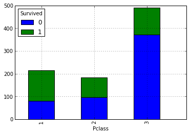
It can be assumed that the higher the social status, the greater the likelihood of salvation. Let's check it out by looking at the number of survivors and drowning depending on the grade. For this you need to build the following summary:
Our above assumption is that the higher their social status among passengers is, the higher is their likelihood of salvation. Now let's take a look at how the number of relatives affects the fact of salvation:
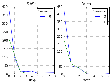
As can be seen from the graphs, our assumption was again confirmed, and not many of the people with more than 1 relatives were saved.
Now we speculate about the data that are cabin numbers. Theoretically, there may not be any data about user cabins, so let's look at this field as much as this one is filled in:
As a result, only 204 records and 890 are filled in, on the basis of this it can be concluded that this field can be omitted during analysis.
The next field that we will analyze will be a field with age ( Age ). Look at how full it is:
This field is almost all filled (714 non-empty records), but there are empty values that are not defined. Let's give it a value equal to the median by age of the entire sample. This step is needed for more accurate model building:
We have left to deal with the fields Ticket , Embarked , Fare , Name . Let's look at the Embarked field, in which the landing port is located, and check if there are any passengers whose port is not listed:
So we found 2 such passengers. Let's assign these passengers the port in which the village has the most people:
Well, we have dealt with one more field and now we have fields with the passenger's name, ticket number and ticket price.
In fact, we need only the price ( Fare ) of these three fields, since it determines to some extent the ranking within the classes of the Pclass field. That is, for example, people inside the middle class can be divided into those who are closer to the first (upper) class, and who are closer to the third (lower) class. Let's check this field for empty values and if any, we will replace the price with the median at the price of all the samples:
In our case there are no empty entries.
In turn, the ticket number and the passenger's name will not help us in any way, since this is just reference information. The only thing for which they can be useful is the definition of which of the passengers are potentially relatives, but since people who have relatives almost did not escape (this was shown above), we can ignore this data.
Now, after removing all unnecessary fields, our set looks like this:
The preliminary analysis of the data is completed, and according to its results, we have obtained a kind of sample, which contains several fields and it would seem possible to break the construction of the model, if not for one “but”: our data contain not only numerical, but also text data.
Therefore, before building a model, you need to encode all our text values.
You can do it manually, or by using the sklearn.preprocessing module. Let's use the second option.
You can encode a list with fixed values using the LabelEncoder () object. The essence of this function is that the input to it is a list of values, which must be encoded, the output is a list of classes whose indices are the codes of the elements of the input list.
As a result, our initial data will look like this:
Now we need to write the code to bring the verification file in the desired form. To do this, you can simply copy the pieces of code that were above (or just write a function to process the input file):
The code described above performs almost the same operations as we did with the training sample. The difference is that a line was added to process the Fare field, if it is not filled out.
Well, the data is processed and you can start building a model, but first you need to decide how we will check the accuracy of the model obtained. For this test, we will use sliding controls and ROC curves . We will perform the test on the training sample, after which we apply it to the test sample.
So consider a few machine learning algorithms:
Let's load the libraries we need:
To begin with, it is necessary to divide our training sample into an indicator that we study, and its defining characteristics:
Now our learning sample looks like this:
Now we divide the indicators obtained earlier into 2 subsamples (training and test) for calculating ROC curves (for sliding control, this is not necessary, since the verification function does it itself. The cross_validation module’s train_test_split function will help us with this:
As parameters, it is passed to:
At the output, the function returns 4 arrays:
Below are the listed methods with the best parameters selected by experience:
Now check the resulting models using the sliding control. To do this, we need to use the cross_val_score function .
Let's look at the graph of the average cross-test tests for each model:
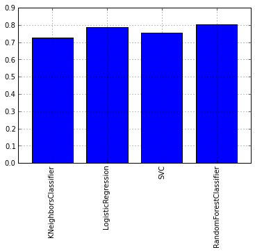
As you can see from the graph, the RandomForest algorithm showed itself best of all. Now let's take a look at the graphs of ROC-curves, to assess the accuracy of the classifier. We will draw graphs using the matplotlib library:
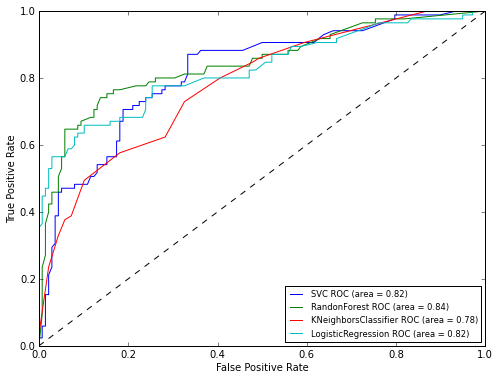
As can be seen from the results of ROC analysis, the best result again showed RandomForest. Now it remains to apply our model to the test sample:
In this article I tried to show how you can use the pandas package in conjunction with the sklearn machine learning package . The resulting model with Kaggle submission showed an accuracy of 0.77033. In the article, I wanted to show more precisely how to work with the tools and the progress of the research, rather than building a detailed algorithm, such as in this series of articles.
Formulation of the problem
So, the essence of the task is to build a model using machine learning methods that predicts whether a person will be saved or not. 2 files are attached to the task:
- train.csv - the data set on the basis of which the model will be built ( training sample )
- test.csv - data set for model checking
As it was written above, for the analysis modules Pandas and scikit-learn will be needed. With Pandas, we will conduct an initial analysis of the data, and sklearn will help in calculating the predictive model. So, first, load the required modules:
In addition, explanations are given for some fields:
- PassengerId - passenger ID
- Survival - a field in which it is indicated that a person was saved (1) or not (0)
- Pclass - contains socio-economic status:
- tall
- average
- low
- Name - passenger's name
- Sex - passenger floor
- Age - age
- SibSp - contains information about the number of second-order relatives (husband, wife, brothers, sets)
- Parch - contains information on the number of relatives on the board of the 1st order (mother, father, children)
- Ticket - ticket number
- Fare - ticket price
- Cabin - Cabin
- Embarked - landing port
- C - Cherbourg
- Q - Queenstown
- S - Southampton
Input analysis
> So, the task is formed and you can begin to solve it.
First, let's load a test sample and see how it looks like:
')
from pandas import read_csv, DataFrame, Series data = read_csv('Kaggle_Titanic/Data/train.csv') | PassengerId | Survived | Pclass | Name | Sex | Age | Sibsp | Parch | Ticket | Fare | Cabin | Embarked |
|---|---|---|---|---|---|---|---|---|---|---|---|
| one | 0 | 3 | Braund, Mr. Owen harris | male | 22 | one | 0 | A / 5 21171 | 7.2500 | NaN | S |
| 2 | one | one | Cumings, Mrs. John Bradley (Florence Briggs Th ... | female | 38 | one | 0 | PC 17599 | 71.2833 | C85 | C |
| 3 | one | 3 | Heikkinen, Miss. Laina | female | 26 | 0 | 0 | STON / O2. 3101282 | 7.9250 | NaN | S |
| four | one | one | Futrelle, Mrs. Jacques Heath (Lily May Peel) | female | 35 | one | 0 | 113803 | 53.1000 | C123 | S |
| five | 0 | 3 | Allen, Mr. William Henry | male | 35 | 0 | 0 | 373450 | 8.0500 | NaN | S |
It can be assumed that the higher the social status, the greater the likelihood of salvation. Let's check it out by looking at the number of survivors and drowning depending on the grade. For this you need to build the following summary:
data.pivot_table('PassengerId', 'Pclass', 'Survived', 'count').plot(kind='bar', stacked=True) Our above assumption is that the higher their social status among passengers is, the higher is their likelihood of salvation. Now let's take a look at how the number of relatives affects the fact of salvation:
fig, axes = plt.subplots(ncols=2) data.pivot_table('PassengerId', ['SibSp'], 'Survived', 'count').plot(ax=axes[0], title='SibSp') data.pivot_table('PassengerId', ['Parch'], 'Survived', 'count').plot(ax=axes[1], title='Parch') As can be seen from the graphs, our assumption was again confirmed, and not many of the people with more than 1 relatives were saved.
Now we speculate about the data that are cabin numbers. Theoretically, there may not be any data about user cabins, so let's look at this field as much as this one is filled in:
data.PassengerId[data.Cabin.notnull()].count() As a result, only 204 records and 890 are filled in, on the basis of this it can be concluded that this field can be omitted during analysis.
The next field that we will analyze will be a field with age ( Age ). Look at how full it is:
data.PassengerId[data.Age.notnull()].count() This field is almost all filled (714 non-empty records), but there are empty values that are not defined. Let's give it a value equal to the median by age of the entire sample. This step is needed for more accurate model building:
data.Age = data.Age.median() We have left to deal with the fields Ticket , Embarked , Fare , Name . Let's look at the Embarked field, in which the landing port is located, and check if there are any passengers whose port is not listed:
data[data.Embarked.isnull()] | PassengerId | Survived | Pclass | Name | Sex | Age | Sibsp | Parch | Ticket | Fare | Cabin | Embarked |
|---|---|---|---|---|---|---|---|---|---|---|---|
| 62 | one | one | Icard, Miss. Amelie | female | 28 | 0 | 0 | 113572 | 80 | B28 | NaN |
| 830 | one | one | Stone, Mrs. George Nelson (Martha Evelyn) | female | 28 | 0 | 0 | 113572 | 80 | B28 | NaN |
So we found 2 such passengers. Let's assign these passengers the port in which the village has the most people:
MaxPassEmbarked = data.groupby('Embarked').count()['PassengerId'] data.Embarked[data.Embarked.isnull()] = MaxPassEmbarked[MaxPassEmbarked == MaxPassEmbarked.max()].index[0] Well, we have dealt with one more field and now we have fields with the passenger's name, ticket number and ticket price.
In fact, we need only the price ( Fare ) of these three fields, since it determines to some extent the ranking within the classes of the Pclass field. That is, for example, people inside the middle class can be divided into those who are closer to the first (upper) class, and who are closer to the third (lower) class. Let's check this field for empty values and if any, we will replace the price with the median at the price of all the samples:
data.PassengerId[data.Fare.isnull()] In our case there are no empty entries.
In turn, the ticket number and the passenger's name will not help us in any way, since this is just reference information. The only thing for which they can be useful is the definition of which of the passengers are potentially relatives, but since people who have relatives almost did not escape (this was shown above), we can ignore this data.
Now, after removing all unnecessary fields, our set looks like this:
data = data.drop(['PassengerId','Name','Ticket','Cabin'],axis=1) | Survived | Pclass | Sex | Age | Sibsp | Parch | Fare | Embarked |
|---|---|---|---|---|---|---|---|
| 0 | 3 | male | 28 | one | 0 | 7.2500 | S |
| one | one | female | 28 | one | 0 | 71.2833 | C |
| one | 3 | female | 28 | 0 | 0 | 7.9250 | S |
| one | one | female | 28 | one | 0 | 53.1000 | S |
| 0 | 3 | male | 28 | 0 | 0 | 8.0500 | S |
Input Preprocessing
The preliminary analysis of the data is completed, and according to its results, we have obtained a kind of sample, which contains several fields and it would seem possible to break the construction of the model, if not for one “but”: our data contain not only numerical, but also text data.
Therefore, before building a model, you need to encode all our text values.
You can do it manually, or by using the sklearn.preprocessing module. Let's use the second option.
You can encode a list with fixed values using the LabelEncoder () object. The essence of this function is that the input to it is a list of values, which must be encoded, the output is a list of classes whose indices are the codes of the elements of the input list.
from sklearn.preprocessing import LabelEncoder label = LabelEncoder() dicts = {} label.fit(data.Sex.drop_duplicates()) # dicts['Sex'] = list(label.classes_) data.Sex = label.transform(data.Sex) # label.fit(data.Embarked.drop_duplicates()) dicts['Embarked'] = list(label.classes_) data.Embarked = label.transform(data.Embarked) As a result, our initial data will look like this:
| Survived | Pclass | Sex | Age | Sibsp | Parch | Fare | Embarked |
|---|---|---|---|---|---|---|---|
| 0 | 3 | one | 28 | one | 0 | 7.2500 | 2 |
| one | one | 0 | 28 | one | 0 | 71.2833 | 0 |
| one | 3 | 0 | 28 | 0 | 0 | 7.9250 | 2 |
| one | one | 0 | 28 | one | 0 | 53.1000 | 2 |
| 0 | 3 | one | 28 | 0 | 0 | 8.0500 | 2 |
Now we need to write the code to bring the verification file in the desired form. To do this, you can simply copy the pieces of code that were above (or just write a function to process the input file):
test = read_csv('Kaggle_Titanic/Data/test.csv') test.Age[test.Age.isnull()] = test.Age.mean() test.Fare[test.Fare.isnull()] = test.Fare.median() # MaxPassEmbarked = test.groupby('Embarked').count()['PassengerId'] test.Embarked[test.Embarked.isnull()] = MaxPassEmbarked[MaxPassEmbarked == MaxPassEmbarked.max()].index[0] result = DataFrame(test.PassengerId) test = test.drop(['Name','Ticket','Cabin','PassengerId'],axis=1) label.fit(dicts['Sex']) test.Sex = label.transform(test.Sex) label.fit(dicts['Embarked']) test.Embarked = label.transform(test.Embarked) The code described above performs almost the same operations as we did with the training sample. The difference is that a line was added to process the Fare field, if it is not filled out.
| Pclass | Sex | Age | Sibsp | Parch | Fare | Embarked |
|---|---|---|---|---|---|---|
| 3 | one | 34.5 | 0 | 0 | 7.8292 | one |
| 3 | 0 | 47.0 | one | 0 | 7.0000 | 2 |
| 2 | one | 62.0 | 0 | 0 | 9.6875 | one |
| 3 | one | 27.0 | 0 | 0 | 8.6625 | 2 |
| 3 | 0 | 22.0 | one | one | 12.2875 | 2 |
Construction of classification models and their analysis
Well, the data is processed and you can start building a model, but first you need to decide how we will check the accuracy of the model obtained. For this test, we will use sliding controls and ROC curves . We will perform the test on the training sample, after which we apply it to the test sample.
So consider a few machine learning algorithms:
Let's load the libraries we need:
from sklearn import cross_validation, svm from sklearn.neighbors import KNeighborsClassifier from sklearn.ensemble import RandomForestClassifier from sklearn.linear_model import LogisticRegression from sklearn.metrics import roc_curve, auc import pylab as pl To begin with, it is necessary to divide our training sample into an indicator that we study, and its defining characteristics:
target = data.Survived train = data.drop(['Survived'], axis=1) # Id kfold = 5 # itog_val = {} # Now our learning sample looks like this:
| Pclass | Sex | Age | Sibsp | Parch | Fare | Embarked |
|---|---|---|---|---|---|---|
| 3 | one | 28 | one | 0 | 7.2500 | 2 |
| one | 0 | 28 | one | 0 | 71.2833 | 0 |
| 3 | 0 | 28 | 0 | 0 | 7.9250 | 2 |
| one | 0 | 28 | one | 0 | 53.1000 | 2 |
| 3 | one | 28 | 0 | 0 | 8.0500 | 2 |
Now we divide the indicators obtained earlier into 2 subsamples (training and test) for calculating ROC curves (for sliding control, this is not necessary, since the verification function does it itself. The cross_validation module’s train_test_split function will help us with this:
ROCtrainTRN, ROCtestTRN, ROCtrainTRG, ROCtestTRG = cross_validation.train_test_split(train, target, test_size=0.25) As parameters, it is passed to:
- Parameter Array
- Array of indicators
- The ratio in which the training set will be split (in our case, 1/4 of the data from the original training set will be allocated to the test set)
At the output, the function returns 4 arrays:
- New learning array of parameters
- test array of parameters
- New array of indicators
- test array of indicators
Below are the listed methods with the best parameters selected by experience:
model_rfc = RandomForestClassifier(n_estimators = 70) # - model_knc = KNeighborsClassifier(n_neighbors = 18) # - model_lr = LogisticRegression(penalty='l1', tol=0.01) model_svc = svm.SVC() # kernek='rbf' Now check the resulting models using the sliding control. To do this, we need to use the cross_val_score function .
scores = cross_validation.cross_val_score(model_rfc, train, target, cv = kfold) itog_val['RandomForestClassifier'] = scores.mean() scores = cross_validation.cross_val_score(model_knc, train, target, cv = kfold) itog_val['KNeighborsClassifier'] = scores.mean() scores = cross_validation.cross_val_score(model_lr, train, target, cv = kfold) itog_val['LogisticRegression'] = scores.mean() scores = cross_validation.cross_val_score(model_svc, train, target, cv = kfold) itog_val['SVC'] = scores.mean() Let's look at the graph of the average cross-test tests for each model:
DataFrame.from_dict(data = itog_val, orient='index').plot(kind='bar', legend=False) As you can see from the graph, the RandomForest algorithm showed itself best of all. Now let's take a look at the graphs of ROC-curves, to assess the accuracy of the classifier. We will draw graphs using the matplotlib library:
pl.clf() plt.figure(figsize=(8,6)) #SVC model_svc.probability = True probas = model_svc.fit(ROCtrainTRN, ROCtrainTRG).predict_proba(ROCtestTRN) fpr, tpr, thresholds = roc_curve(ROCtestTRG, probas[:, 1]) roc_auc = auc(fpr, tpr) pl.plot(fpr, tpr, label='%s ROC (area = %0.2f)' % ('SVC', roc_auc)) #RandomForestClassifier probas = model_rfc.fit(ROCtrainTRN, ROCtrainTRG).predict_proba(ROCtestTRN) fpr, tpr, thresholds = roc_curve(ROCtestTRG, probas[:, 1]) roc_auc = auc(fpr, tpr) pl.plot(fpr, tpr, label='%s ROC (area = %0.2f)' % ('RandonForest',roc_auc)) #KNeighborsClassifier probas = model_knc.fit(ROCtrainTRN, ROCtrainTRG).predict_proba(ROCtestTRN) fpr, tpr, thresholds = roc_curve(ROCtestTRG, probas[:, 1]) roc_auc = auc(fpr, tpr) pl.plot(fpr, tpr, label='%s ROC (area = %0.2f)' % ('KNeighborsClassifier',roc_auc)) #LogisticRegression probas = model_lr.fit(ROCtrainTRN, ROCtrainTRG).predict_proba(ROCtestTRN) fpr, tpr, thresholds = roc_curve(ROCtestTRG, probas[:, 1]) roc_auc = auc(fpr, tpr) pl.plot(fpr, tpr, label='%s ROC (area = %0.2f)' % ('LogisticRegression',roc_auc)) pl.plot([0, 1], [0, 1], 'k--') pl.xlim([0.0, 1.0]) pl.ylim([0.0, 1.0]) pl.xlabel('False Positive Rate') pl.ylabel('True Positive Rate') pl.legend(loc=0, fontsize='small') pl.show() As can be seen from the results of ROC analysis, the best result again showed RandomForest. Now it remains to apply our model to the test sample:
model_rfc.fit(train, target) result.insert(1,'Survived', model_rfc.predict(test)) result.to_csv('Kaggle_Titanic/Result/test.csv', index=False) Conclusion
In this article I tried to show how you can use the pandas package in conjunction with the sklearn machine learning package . The resulting model with Kaggle submission showed an accuracy of 0.77033. In the article, I wanted to show more precisely how to work with the tools and the progress of the research, rather than building a detailed algorithm, such as in this series of articles.
Source: https://habr.com/ru/post/202090/
All Articles