Motion planning: visibility graph, road maps

Good day everyone. In this article I would like to tell you about a couple of algorithms related to computational geometry, which are currently widely used in game development. If you at least once programmed a game in which there is a character (s) moving in a location, you had to solve the task of finding a path. On one of the approaches to solving this problem and I want to tell.

Formulation of the problem

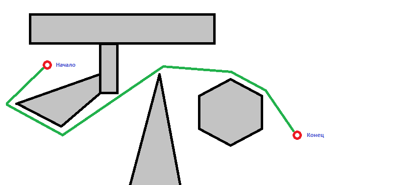
Let a set of non-intersecting polygons of P - polygonal obstacles be given. Let there be an agent moving in the same plane - it is represented by a point. Let start point s and end point f be given. We need to build the shortest route from point s to point f, while we assume that the agent may be on the border of the obstacle, but not inside it.

Decision

Optimal way

It can be proved that the optimal path is a piecewise linear broken line whose vertices coincide with the vertices of the obstacles.

Evidence

Part 1. The optimal path is a piecewise linear broken line.
')
Suppose that the shortest path T is not a piecewise linear broken line. In this case, on the path T, there exists a point p that does not belong to any direct segment of T (Figure 1). This means that there is an ε-neighborhood of the point p (Figure 2) into which no obstacle falls. In this case, the subtrail T _ε , which is inside the ε-neighborhood, can be shortened along a chord, connecting the intersection points of the ε-neighborhood with the path T. Since part of the path can be reduced, this means that the whole path can be reduced, and therefore the assumption is incorrect. Path T is a piecewise linear broken line.


Figure 1. Point p on path T	Figure 2. The ε-neighborhood of the point p	Figure 3. Chord, which is the shortest path

Part 2. The tops of the path coincide with the tops of the obstacles.
Suppose now that the vertices of the path T do not coincide with the vertices of the obstacle polygons. Consider the vertex v of the path T. The vertex cannot lie inside the free space, because otherwise, using a similar approach, we would find a shorter path along the chord in the ε-neighborhood of the vertex v (Figure 4). Therefore, the vertex v must lie on the boundaries of the obstacles (at their vertices or on the edges). But the vertex cannot lie on the edges either, since (again we consider the ε-neighborhood), we can cut along the chord (Figure 5).


Figure 4. ε-neighborhood of the top of the path lying in a free space	Figure 5. ε-neighborhood of the top of the path lying on the edge

The above means that the vertices of the piecewise linear path T must be located at the vertices of the obstacles-polygons.

Graph of visibility

We will call two points mutually visible if the segment connecting them does not contain internal points of obstacles-polygons.
To build the shortest path is used visibility graph. The vertices of the graph are the vertices of the obstacles-polygons. The edges are connected only mutually visible vertices of the graph.

Figure 6. Example of a visibility graph.

Suppose we have built the visibility graph VG. Add to the graph VG the vertices s and f, as well as the edges connecting them with all the visible vertices of them. We obtain the extended graph VG ⁺ . We will only need to find the shortest path from the vertex s to the vertex f in the graph VG ⁺ . This can be done by applying the Dijkstra algorithm . I will not talk in detail about it, because on the Internet there are a huge variety of articles, including on Habré . It remains only to solve the problem of constructing the graph of visibility.

Visibility graph construction: naive algorithm

We will iterate over all pairs of vertices in the VG ⁺ graph and check for each of them whether the segment connecting the vertices of the obstacle edge does not intersect. It is easy to see that the complexity of such an algorithm is O (n ³ ), since we have n ² pairs of vertices and O (n) edges.

Construction of visibility graph for O (n ² log (n))

Let's try to build a graph of visibility a little faster. For each vertex, we find all the vertices visible from it using the plane sweep method. We need to solve the following problem: a set of segments (obstacle edges) and a point p are given on the plane. Find all the ends of the segments visible from point p. We will sweep the plane with a rotating beam starting at the point p (Figure 7). The status of a sweeping straight line will be the segments that intersect it, ordered in increasing distance from the point p to the intersection point. The event points will be the ends of the segments.

Figure 7. Observing a plane by a rotating beam.

Ordered by angle relative to the axis passing through point p vertices will be stored in the event queue. The status initialization takes O (nlog (n)) time, the event queue initialization also takes O (nlog (n)) time. The total running time of the sweep algorithm is O (nlog (n)), thus, applying the algorithm for each vertex of the graph, we obtain the visibility graph in a time of order O (n ² log (n)).
More formally. Let the number of edges of the set of non-intersecting polygons-obstruction be n. In the spoilers, I will give the code in a pseudo-language, most similar to Java.

Building visibility graph

public final G buildVisibilityGraph(final Set<Segment> segments) { /*  .        .   - . */ final G visibilityGraph = new G(getVertices(segments)); /*     */ for (final Vertex v : visibilityGraph.getVertices()) { /*       */ final Set<Vertex> visibleVertices = getVisibleVertices(v, segments); /*       */ for (final Vertex w : visibleVertices) visibilityGraph.addEdge(v, w); } return visibilityGraph; }

The buildVisibilityGraph function takes as input a set of segments — the edges of the obstacle polygons and returns the constructed visibility graph. Explanations here, it seems to me, are not required. Consider the pseudo-code of the getVisibleVertices function.

Listing all visible vertices

 public final Set<Vertex> getVisibleVertices(final Vertex v, final Set<Segment> segments) { /*    ( )  ,   pw ( w -  )   ,    v */ final SortedSet<Vertex> sortedVertices = sortSegmentsVertices(v, segments); /*  I -  ,   v.   ,                   */ final BST<Segment> intersectedSegments = new BST<Segment>(v, segments); /*     */ final Set<Vertex> visibleVertices = new HashSet<Vertex>(); /*     */ for (final Vertex w : sortedVertices) { if (isVertexVisible(v, w, intersectedSegments)) visibleVertices.add(w); /*      ,   w       ( vw),  ,    w */ intersectedSegments.add(getIncidentSegments(v, w, Position.RightOf)); /*      ,   w       ( vw),  ,    w */ intersecedSegments.remove(getIncidentSegments(v, w, Position.LeftOf)); } return visibleVertices; }

So, the first thing vertices w ∈ W are sorted by the angle between the ray vw and the vertical semi-axis passing through v. This sorting is done in O (nlog (n)), for example, by merging sorting. Then the set of visible vertices is initialized (by default, such a set is empty). Next begins sweeping the plane. In the sort order of the vertices, each of them is checked: is the vertex w visible from the vertex v. Since such a check means the presence of intersections that are stored in a balanced tree, it can be performed in O (log (n)). If the vertex is visible, you need to add it to the list of visible vertices. And finally, regardless of the visibility of the vertex, it is necessary to change the status of the sweeping line. To do this, for the current vertex w, you must remove from the list of current intersections all edges (segments) that end at this vertex (lie to the left of the line vw) and add all edges (segments) that start at it (lie to the right of the line vw) .
Consider Figures 8-10:

Figures 8-10

Figure 8. Step 1. Updating the status of a sweeping straight.

Figure 9. Step 2. Updating the status of a sweeping straight.

Figure 10. Step 3. Updating the status of a sweeping straight.

So, in the first step (ray vw ₁ ), two segments w ₁ w ₅ and w ₁ w ₂ are added to the tree, since they lie to the right of the ray vw ₁ . The status of the sweeping line is marked in orange.
In the second step (the second vertex in the list is the vertex w ₃ ), two more edges are added to the status: w ₃ w ₂ and w ₃ w ₄ . Now in the status are 4 edges. Finally, at the third step (vertex w ₂ ), 2 edges are removed from the status: w ₃ w ₂ and w ₁ w ₂ .

Ultimately, you should look at the function of checking the visibility of the vertex.

Vertex visibility function

 public final boolean isVisible(final Vertex v, final Vertex w, final BST<Vertex> intersections) { final Segment currentSegment = new Segment(v, w); /*  vw    ,   w,    */ if (intersects(currentSegment, w.getSegments()) return false; /*   ( )    vw. */ if (currentSegment.contains(w.getPreviousVertex())) { /*   ,  ,   */ if (!v.getPreviousVertex().isVisible()) return false; return !intersections.hasIntersectionsWith(new Segment(w.getPrevious(), w)); } /*         (    vw    ) */ return intersections.intersectWithLeftMost(currentSegment); }

This function should only return true if the vertex w is visible from the vertex v and false otherwise. To do this, it is enough just to compare the length of the segment vw and the distance from the point v to the intersection with the nearest segment stored in the tree (the leftmost sheet). But there are several marginal cases:

The ray vw intersects the edges incident to the vertices v or w
The ray coincides with the edge on which there are other vertices.

Thus, the visibility check function works in the worst case for O (log (n)), because it uses search in a balanced tree. The remaining operations are performed in constant time.

Road maps

Another route planning method is the use of road maps. Sounds like a truism, doesn't it? In this article, I will briefly talk about its essence (because the article is already quite voluminous), if anyone is interested, I will probably write another publication later. So.

We construct a rectangle containing all the polygons-obstacles inside (figure 11). Consider the set of segments - the edges of the obstacles and construct a trapezoidal map for it (Figure 12), and then remove from the resulting map all the trapezoids lying inside the obstacles (Figure 13). It takes O (nlog (n)) time to build a map, where n is the total number of obstacle vertices. In order to decide whether to remove the trapezoid T, it suffices to take the edge top (T) and check whether an obstacle lies above or below it, the boundary of which contains this edge. Thus, it will take O (n) time to remove all the extra trapezoids.
If the starting and ending points are inside one trapezoid, then you can pass from the first point to the second in a straight line. If these points lie in different trapezoid, then the path will cross several trapezoids, and, probably, in some of them we will have to make turns.
We construct a road map — graph G. The vertices of G are the midpoints of the vertical line segments drawn through the tops of the obstacles and the midpoints of the trapezoids. Two vertices of the graph G are connected by an edge if and only if one of them is the middle of some trapezoid, and the other lies on the vertical edge of this trapezoid. The graph G can be constructed from a trapezoidal map in time O (n). Note that the graph G is a planar graph.
In order to find a path from point s to point f, we first determine which trapezoid contains s and f. If they got into one trapezoid, then the shortest path is a straight line. Otherwise, we move in a straight line from point s to the middle of the trapezoid containing it, then move along the edges of the graph to the middle of the trapezoid containing point f (you can use wide search), and finally move to point f in a straight line from the middle of the trapezoid containing it (figure 14). Since the trapezoidal map contains a linear number of trapezoids in n, and the number of segments of vertical lines drawn through the vertices of the obstacles is also linear in n, the graph G has O (n) vertices, and since it is planar, the number of edges is also O ( n). Therefore, a wide search on G can be performed in O (n) time. Since localization of a point in the trapezoidal map takes O (log (n)) time, it takes O (n) to build a path from point s to point f. But the paths constructed using roadmaps will not be optimal.


Figure 11. Building an enclosing rectangle	Figure 12. Trapezoidal map	Figure 13. Reduced trapezoidal map

Figure 14. Built road map

Subtasks

Constructing a convex hull

In general, a scene is a collection of arbitrary objects. For each of them, a convex hull can be constructed (well, or a bounding volume, if greater precision is not needed, or all objects resemble rectangles). In order to be able to use the visibility graph for arbitrary geometry, it is necessary to map it to the set of polygons. The simplest method is to construct a convex hull. There are several different algorithms for its construction and this is a topic for a separate article, I just mention them here:

Naive algorithm. Works for O (n ⁴ ). For each “not extreme” (that is, such a point of a set through which a straight line can be drawn, relative to which the whole set will lie on one side), the following test is performed. If it belongs to at least one triangle obtained from the points of the set, then it is a point of a convex hull. In the set of N points N ³ triangles. Therefore for each of the N points you need to perform N ³ checks.
Slightly less naive algorithm. O (n ³ ). A complete graph is constructed with a set of nodes — the points of the original set. For each edge (of which N ² ) the remaining N-2 points are checked. Do they all lie on one side of this edge. If so, then the edge belongs to the convex hull.
Jarvis algorithm. Works for O (n ² ). Imagine a lot of points on a plane. Choose the leftmost among them (this can always be done (if there are several, then any among the left), it is obviously a point of a convex hull), and then “wrap” the set as a gift. Among all the other points we choose the one that has the smallest polar angle (by analogy with the construction of the visibility graph, we sweep it with a ray)
Graham's Algorithm. Works for O (nlog (n)). I will not provide the description (as you understand, the faster the algorithm, the more scribbling) - google

Intersection of segments

Finally, the last task that needs to be solved in the construction of the visibility graph is to check two segments for intersections. This is a very good topic for a separate article, since there is also a lot of writing on this issue. I just give you one of the methods for solving the problem that I like : here it is .

Conclusion

I hope someone article seemed interesting, and maybe even useful. In the near future I plan to publish another article, and then we will see - let's arrange a survey on whether to continue.

Instead of a thousand words

Motion planning: visibility graph, road maps

Formulation of the problem

Decision

Optimal way

Figure 1. Point p on path T

Figure 2. The ε-neighborhood of the point p

Figure 3. Chord, which is the shortest path

Figure 4. ε-neighborhood of the top of the path lying in a free space

Figure 5. ε-neighborhood of the top of the path lying on the edge

Graph of visibility

Figure 6. Example of a visibility graph.

Visibility graph construction: naive algorithm

Construction of visibility graph for O (n ² log (n))

Figure 7. Observing a plane by a rotating beam.

Figure 8. Step 1. Updating the status of a sweeping straight.

Figure 9. Step 2. Updating the status of a sweeping straight.

Figure 10. Step 3. Updating the status of a sweeping straight.

Road maps

Figure 11. Building an enclosing rectangle

Figure 12. Trapezoidal map

Figure 13. Reduced trapezoidal map

Figure 14. Built road map

Subtasks

Constructing a convex hull

Intersection of segments

Conclusion

Links

More articles:

Motion planning: visibility graph, road maps

Formulation of the problem

Decision

Optimal way

Figure 1. Point p on path T

Figure 2. The ε-neighborhood of the point p

Figure 3. Chord, which is the shortest path

Figure 4. ε-neighborhood of the top of the path lying in a free space

Figure 5. ε-neighborhood of the top of the path lying on the edge

Graph of visibility

Figure 6. Example of a visibility graph.

Visibility graph construction: naive algorithm

Construction of visibility graph for O (n 2 log (n))

Figure 7. Observing a plane by a rotating beam.

Figure 8. Step 1. Updating the status of a sweeping straight.

Figure 9. Step 2. Updating the status of a sweeping straight.

Figure 10. Step 3. Updating the status of a sweeping straight.

Road maps

Figure 11. Building an enclosing rectangle

Figure 12. Trapezoidal map

Figure 13. Reduced trapezoidal map

Figure 14. Built road map

Subtasks

Constructing a convex hull

Intersection of segments

Conclusion

Links

More articles:

Construction of visibility graph for O (n ² log (n))