Speech recognition from Yandex. Under the hood of Yandex.SpeechKit

At the Yet Another Conference 2013, we presented our new Yandex SpeechKit library to developers. This is a public speech recognition API that Android and iOS developers can use. Download SpeechKit, as well as get acquainted with the documentation, here .

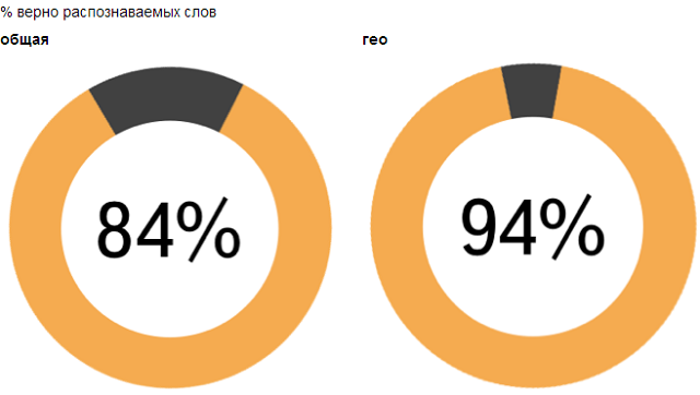
Yandex SpeechKit allows you to directly access that backend, which is successfully used in Yandex mobile applications. We have been developing this system for quite a long time and now correctly recognize 94% of words in Navigator and Mobile Maps, as well as 84% ​​of words in Mobile Browser. In this case, recognition takes a little more than a second. This is a very decent quality, and we are actively working to improve it.


')
It can be argued that very soon the voice interfaces will practically not differ in reliability from the classical input methods. Detailed story about how we managed to achieve such results, and how our system is arranged, under the cut.



Speech recognition is one of the most interesting and challenging tasks of artificial intelligence. It involves the achievement of very different areas: from computational linguistics to digital signal processing. In order to understand how a machine should be arranged, an understanding speech, let us first understand what we are dealing with.

I. Basics

For us, sounding speech is, first of all, a digital signal. And if we look at the recording of this signal, we will not see there either words or clearly pronounced phonemes - various “speech events” smoothly flow into each other, without forming clear boundaries. The same phrase, pronounced by different people or in different settings, at the signal level will look different. At the same time, people somehow recognize each other's speech: therefore, there are invariants, according to which the signal can be restored, what was actually said. The search for such invariants is the task of acoustic modeling.

Suppose that a person’s speech consists of phonemes (this is a gross simplification, but in the first approximation it is true). Let us define a phoneme as the minimum distinctive unit of a language, that is, a sound, the replacement of which can lead to a change in the meaning of a word or phrase. Take a small section of the signal, say, 25 milliseconds. Let's call this site “frame”. What phoneme was pronounced on this frame? It is difficult to answer this question unequivocally - many phonemes are extremely similar to each other. But if it is impossible to give an unambiguous answer, then one can reason in terms of “probabilities”: for a given signal, some phonemes are more likely, others are less, and still others can be excluded from consideration. Actually, the acoustic model is a function that accepts a small portion of the acoustic signal (frame) and outputs a probability distribution of various phonemes on this frame. Thus, the acoustic model gives us the opportunity to recover from the sound that was said - with varying degrees of confidence.

Another important aspect of acoustics is the probability of transition between different phonemes. We know from experience that some combinations of phonemes are pronounced easily and occur frequently, others are more difficult to pronounce and are used less frequently in practice. We can summarize this information and take it into account when assessing the "plausibility" of a particular sequence of phonemes.

Now we have all the tools to construct one of the main “workhorses” of automatic speech recognition - the hidden Markov Model (HMM, Hidden Markov Model). To do this, for the time being we imagine that we are not solving the problem of speech recognition, but the exact opposite - text-to-speech. Suppose we want to get the pronunciation of the word "Yandex". Let the word “Yandex” consist of a set of phonemes, say, [i] [a] [n] [d] [e] [k] [s]. Construct a finite state machine for the word “Yandex”, in which each phoneme is represented by a separate state. At each moment of time, we are in one of these states and “pronounce” the sound characteristic of this phoneme (how to pronounce each of the phonemes, we know from the acoustic model). But some phonemes last for a long time (as [a] in the word “Yandex”), others are practically swallowed. Here we will need information about the probability of transition between phonemes. Having generated a sound corresponding to the current state, we make a probabilistic decision: remain with us in the same state or proceed to the next (and, accordingly, the next phoneme).



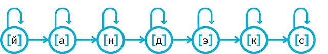
More formally, the HMM can be represented as follows. First, we introduce the notion of emission. As we remember from the previous example, each of the states of the HMM "generates" a sound characteristic of this state (i.e., phonemes). At each frame, the sound is “played out” from the probability distribution corresponding to the given phoneme. Secondly, transitions are possible between states, also subject to predetermined probabilistic patterns. For example, the probability that the phoneme [a] will “drag on” is high, which cannot be said about the phoneme [e]. The emission matrix and transition matrix uniquely define the hidden Markov model.

Well, we looked at how hidden Markov model can be used to generate speech, but how to apply it to the inverse problem - speech recognition? Viterbi algorithm comes to the rescue. We have a set of observables (actually, sound) and a probabilistic model that relates hidden states (phonemes) and observables. The Viterbi algorithm allows you to recover the most likely sequence of hidden states.

Let there be only two words in our recognition dictionary: “Yes” ([d] [a]) and “No” ([n '] [e] [t]). Thus, we have two hidden Markov models. Next, let us have a voice recording of a user who says “yes” or “no.” The Viterbi algorithm will allow us to get an answer to the question, which of the recognition hypotheses is more likely.

Now our task is to restore the most probable sequence of states of the hidden Markov model, which “spawned” (more precisely, could have generated) the audio recording presented to us. If the user says "yes", then the corresponding state sequence on 10 frames may be, for example, [d] [d] [d] [d] [a] [a] [a] [a] [a] [a] or [d] [a] [a] [a] [a] [a] [a] [a] [a] [a]. Similarly, different pronunciation options for “no” are possible - for example, [n '] [n'] [n '] [e] [e] [e] [e] [t] [t] [t] and [n' ] [n '] [e] [e] [e] [e] [e] [e] [m] [m]. Now we find the “best”, that is, the most likely, way to pronounce each word. At each frame, we will ask our acoustic model how likely it is that a particular phoneme sounds here (for example, [g] and [a]); in addition, we will take into account the transition probabilities ([g] -> [g], [g] -> [a], [a] -> [a]). So we get the most likely way to pronounce each of the hypothesis words; moreover, for each of them we get a measure, how likely it is that this particular word was pronounced (we can consider this measure as the length of the shortest path through the corresponding graph). The "winning" (i.e. more likely) hypothesis will be returned as a result of recognition.

The Viterbi algorithm is fairly simple to implement (dynamic programming is used) and works in a time proportional to the product of the number of HMM states and the number of frames. However, it is not always enough for us to know the most probable way; For example, when training an acoustic model, an estimate of the probability of each state on each frame is needed. For this, the Forward-Backward algorithm is used.

However, the acoustic model is just one of the components of the system. What to do if the recognition dictionary consists not of two words, as in the above example, but of hundreds of thousands or even millions? Many of them will be very similar in pronunciation or even match. However, in the presence of context, the role of acoustics falls: vaguely pronounced, noisy or ambiguous words can be restored "in meaning." Again, contextual models are again used to take into account the context. For example, the speaker of the Russian language understands that the naturalness (in our case, probability) of the sentence “mom washed the frame” is higher than “mom washed the cyclotron” or “mom washed the frame”. That is, the presence of a fixed context “soap mom ...” sets the probability distribution for the next word, which reflects both semantics and morphology. This type of language model is called n-gram language models (trigrams in the above example); Of course, there are much more complex and powerful ways of modeling a language.

Ii. What is under the hood of Yandex ASR?

Now, when we imagine a common device of speech recognition systems, let us describe in more detail the details of the Yandex technology - the best, according to our data, Russian speech recognition systems.
When considering the toy examples above, we intentionally made several simplifications and omitted a number of important details. In particular, we argued that the main "building block" of speech is the phoneme. In fact, the phoneme is too large a unit; To adequately simulate the pronunciation of a single phoneme, three separate states are used - the beginning, the middle and the end of the phoneme. Together they form the same HMM as presented above. In addition, phonemes are position-dependent and context-dependent: formally, the “same” phoneme sounds significantly differently depending on which part of the word it is in and adjacent to which phonemes. At the same time, a simple listing of all possible options for context-sensitive phonemes will return a very large number of combinations, many of which are never found in real life; To make the number of acoustic events considered reasonable, close context-sensitive phonemes are combined in the early stages of the training and are considered together.
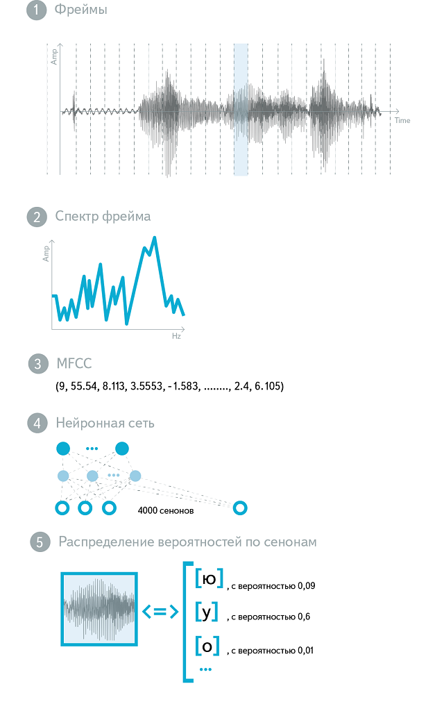
Thus, we, first, made the phonemes context-sensitive, and second, we divided each of them into three parts. These objects - "parts of phonemes" - now make up our phonetic alphabet. They are also called senons. Every state of our HMM is a Senon. Our model uses 48 phonemes and about 4000 cenons.

So, our acoustic model still accepts sound at the input, and the output gives a probability distribution over the senons. Now consider what exactly is fed to the input. As we said, the sound is cut in sections of 25 ms ("frames"). Typically, the cutting pitch is 10 ms, so that the adjacent frames overlap partially. It is clear that the "raw" sound - the amplitude of oscillations in time - not the most informative form of the representation of the acoustic signal. The spectrum of this signal is already much better. In practice, the logarithm and scaled spectrum is usually used, which corresponds to the laws of human hearing ( Mel-transformation ). The values ​​obtained are subjected to discrete cosine transform ( DCT ), and the result is the MFCC - Mel Frequency Cepstral Coefficients. (The word Cepstral is obtained by rearranging the letters in Spectral, which reflects the presence of an additional DCT). MFCC is a vector of 13 (usually) real numbers. They can be used as an input to the “raw” acoustic model, but more often they undergo many additional transformations.

Training an acoustic model is a complex and multi-step process. Expectation-Maximization family algorithms are used for training , such as the Baum-Welch algorithm . The essence of such algorithms is in the alternation of two steps: in the Expectation step, the existing model is used to calculate the expectation of the likelihood function, in the Maximization step, the model parameters are changed in such a way as to maximize this estimate. In the early stages of the training, simple acoustic models are used: simple MFCC features are given at the input, phonemes are considered out of context, and the HMM uses a mixture of Gaussian diagonal GMMs (Gaussian Mixture Models) to model the probability of emission. The results of each previous acoustic model are the starting point for training a more complex model, with a more complex input, output or emission probability distribution function. There are many ways to improve the acoustic model, but the most significant effect is the transition from the GMM model to the DNN ( Deep Neural Network ), which improves the quality of recognition almost twice. Neural networks are devoid of many of the limitations characteristic of Gaussian mixtures, and have a better generalizing ability. In addition, acoustic models on neural networks are more resistant to noise and have better performance.

The neural network for acoustic modeling is trained in several stages. To initialize the neural network, a stack of Boltzmann Machines (RBM) is used. RBM is a stochastic neural network that trains without a teacher. Although the weights that she learned cannot be directly used to distinguish between classes of acoustic events, they reflect the structure of speech in detail. You can treat RBM as a feature extractor - the resulting generative model turns out to be an excellent starting point for building a discriminative model. A discriminative model is trained using the classical error back-propagation algorithm, and a number of techniques are used to improve convergence and prevent overfitting. As a result, at the input of the neural network there are several frames of MFCC-features (the central frame is subject to classification, the others form the context), and at the output there are about 4000 neurons corresponding to different senons. This neural network is used as an acoustic model in a production system.



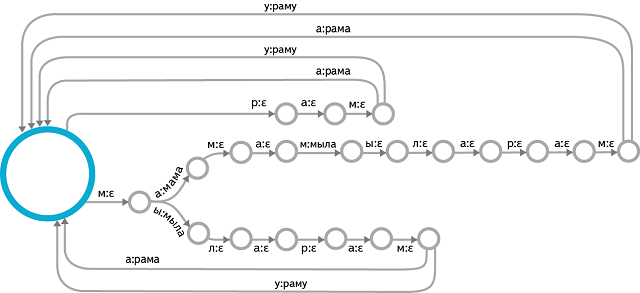
Let's take a closer look at the decoding process. For the problem of recognition of spontaneous speech with a large vocabulary, the approach described in the first section is not applicable. A data structure is needed, connecting together all possible sentences that the system can recognize. A suitable structure is a weighted finite-state transducer (WFST) - in fact, just a finite state machine with output tape and scales on the edges. At the entrance of this machine - Senona, at the exit - the words. The decoding process boils down to choosing the best path in this automaton and providing the output sequence of words corresponding to this path. In this case, the price of passage in each arc consists of two components. The first component is known in advance and is calculated at the assembly stage of the machine. It includes the cost of pronunciation, transition to this state, assessment of the likelihood from the language model. The second component is calculated separately for a specific frame: this is the acoustic weight of the Senon corresponding to the input symbol of the arc in question. Decoding occurs in real time, so not all possible paths are explored: special heuristics limit the set of hypotheses to the most likely ones.

Of course, the most interesting part from a technical point of view is the construction of such an automaton. This problem is solved offline. To go from simple HMM for each context-dependent phoneme to linear automata for each word, we need to use a vocabulary of pronunciations. Creating such a dictionary is impossible manually, and here methods of machine learning are used (and the task itself in the scientific community is called Grapheme-To-Phoneme, or G2P). In turn, the words “dock” with each other into a language model, also represented as a finite state machine. The central operation here is the composition of the WFST, but various methods of optimizing the WFST in terms of size and efficiency of packing in memory are also important.



The result of the decoding process is a list of hypotheses that can be further processed. For example, you can use a more powerful language model to re-rank the most likely hypotheses. The resulting list is returned to the user, sorted by the value of confidence - the degree of our confidence that the recognition passed correctly. Often there is only one hypothesis, in this case, the client application immediately switches to the execution of the voice command.

In conclusion, let us touch on the question of the quality metrics of speech recognition systems. The most popular metric is Word Error Rate (and the opposite of Word Accuracy). Essentially, it reflects the proportion of incorrectly recognized words. To calculate the Word Error Rate for a speech recognition system, manually tagged voice query shells are used that correspond to the subject of an application that uses speech recognition.

Related literature:

1. Mohri, M., Pereira, F., & Riley, M. (2008). Speech recognition with weighted finite-state transducers. In Springer Handbook of Speech Processing (pp. 559-584). Springer Berlin Heidelberg.
2. Hinton, G., Deng, L., Yu, D., Dahl, GE, Mohamed, AR, Jaitly, N. et al. (2012). He has a wide range of research and development programs. Signal Processing Magazine, IEEE, 29 (6), 82-97.
3. Jurafsky D., Martin JH (2008) Speech and language processing, 2nd edition. Prentice Hall.