On a singularity of the Kotelnikov theorem

I was inspired to write this article by the following task:

As is known from Kotelnikov's theorem, in order for an analog signal to be digitized and then reconstructed, it is necessary and sufficient that the sampling frequency be greater than or equal to twice the upper frequency of the analog signal. Suppose we have a sine with a period of 1 second. Then f = 1 ∕ T = 1 hertz, sin ((2 ∗ π T) ∗ t) = sin (2 ∗ π ∗ t), the sampling frequency is 2 hertz, the sampling period is 0.5 seconds. Substitute values ​​that are multiples of 0.5 seconds into the formula for sin: sin (2 ∗ π ∗ 0) = sin (2 ∗ π ∗ 0.5) = sin (2 ∗ π ∗ 1) = 0
Everywhere get zeros. How, then, can this sine be restored?


')
An Internet search did not give an answer to this question, the maximum of what could be found is various discussions on forums where quite bizarre arguments for and against were given before references to experiments with various filters. It should be pointed out that Kotelnikov's theorem is a mathematical theorem and it should be proved or disproved only by mathematical methods. What I did. It turned out that the evidence of this theorem in various textbooks and monographs is quite a lot, but I did not manage to find where this contradiction arises for a long time, because the evidence was presented without many subtleties and details. I will also say that the very formulation of the theorem was different in different sources. Therefore, in the first section I will give a detailed proof of this theorem, following the original work of the academician himself (V.A. Kotelnikov 'On the transmission capacity of the' ether 'and wire in telecommunications.' Materials for the I All-Union Congress on technical reconstruction of communications and the development of low-current industry 1933)

We formulate a theorem as given in the original source:
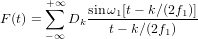
Any function F (t), consisting of frequencies from 0 to f1 periods per second, can be represented next



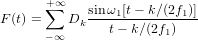
where k is an integer; ω = 2πf1; Dk - constants depending on F (t).

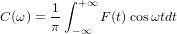
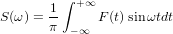
Proof: Any function F (t) that satisfies Dirichlet conditions (a finite number of maxima, minima and break points on any finite segment) and integrable from −∞ to + ∞, which occurs in electrical engineering, can be represented by a Fourier integral:



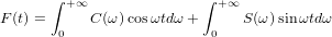
those. as the sum of an infinite number of sinusoidal oscillations with frequencies from 0 to + ∞ and amplitudes of C (ω) dω and S (ω) dω, depending on the frequency. And



In our case, when F (t) consists only of frequencies from 0 to f1, obviously



at



and therefore F (t) can be represented as:



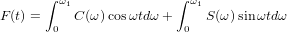
the functions C (ω) and S (ω), like all the others in the segment



can be represented always by Fourier series, and these series can, according to our desire, consist of cosines or sines alone, if we take for the period the double length of the segment, i.e. 2ω1.

Author's note: here it is necessary to give an explanation. Kotelnikov uses the ability to complement the functions C (ω) and S (ω) so that C (ω) becomes even, and S (ω) is an odd function on the double segment with respect to ω1. Accordingly, in the second half of the section, the values ​​of these functions will be C (2 ∗ ω1 −ω) and −S (2 ∗ ω1 −ω). These functions are reflected along the vertical axis with the coordinate ω1, and the function S (ω) also changes the sign

In this way



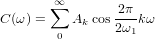
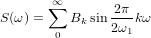
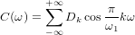
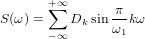
We introduce the following notation.



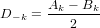
Then



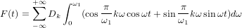
Substituting we get:



Transform



Transform



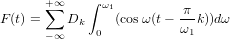
We integrate and replace ω1 by 2πf1:

Inaccuracy in the Kotelnikov theorem

All evidence seems rigorous. What is the problem? To understand this, we turn to one not very well-known property of the inverse Fourier transform. It says that during the inverse transformation from the sum of sines and cosines into the original function, the value of this function will be



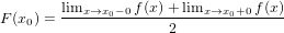
that is, the restored function is equal to the half-sum of the values ​​of the limits. What does this lead to? If our function is continuous, then to nothing. But if there is a final discontinuity in our function, then the function values ​​after the direct and inverse Fourier transforms will not match the original value. Let us now recall a step in the proof of the theorem, where the interval is doubled. The function S (ω) is complemented by the function −S (2 ∗ ω1 - ω). If S (ω1) (the value at the point ω1) is zero, nothing bad happens. However, if the value of S (ω1) is not zero, the reconstructed function will not be equal to the original one, since at this point a discontinuity of 2S (ω1) occurs.
We now return to the original problem about the sine. As is known, the sine is an odd function whose image after the Fourier transform is δ (ω - Ω0) - the delta function. That is, in our case, if the sine has a frequency ω1, we get:



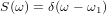
Obviously, at the point ω1, we add two delta functions of S (ω) and −S (ω), forming a zero, which we observe.

Conclusion

The Kotelnikov theorem is undoubtedly a great theorem. However, it must be supplemented by another condition, namely



In such a formulation, boundary cases are excluded, in particular, a case with a sine whose frequency is equal to the boundary frequency ω1, since for him the Kotelnikov theorem with the above condition cannot be used.