Simple words about Fourier transform
I suppose that everyone in general knows about the existence of such a wonderful mathematical tool as the Fourier transform. However, in universities, for some reason, it is taught so poorly that they understand how this transformation works and how they should be used by relatively few people. Meanwhile, the math of this transformation is surprisingly beautiful, simple and elegant. I invite everyone to learn a little more about the Fourier transform and the topic close to him about how analog signals can be effectively converted to digital computing for computational processing.
 (c) xkcd
Without using complex formulas and hardware, I will try to answer the following questions:
')
I will proceed from the assumption that the reader understands what an integral is , a complex number (as well as its module and argument ), convolution of functions , plus at least “on fingers” imagine what the Dirac delta function is . Do not know - it does not matter, read the above links. By “product of functions” in this text I will always understand “pointwise multiplication”
We must begin, probably, from the fact that the usual Fourier transform is some kind of thing that, as the name suggests, converts some functions to others, that is, assigns its spectrum or Fourier transform y to each function of a real variable x (t) (w):

If we give analogies, then an example of a transformation similar in meaning can be, for example, a differentiation that turns a function into its derivative. That is, the Fourier transform is the same, in essence, an operation as the taking of a derivative, and it is often denoted in a similar way, drawing a triangular “cap” over the function. But unlike differentiation, which can be defined for real numbers, the Fourier transform always “works” with more general complex numbers. Because of this, there are always problems with the display of the results of this transformation, since the complex numbers are determined not by one, but by two coordinates on a graph operating with real numbers. Most conveniently, as a rule, it turns out to present complex numbers as a module and argument and draw them separately as two separate graphs:
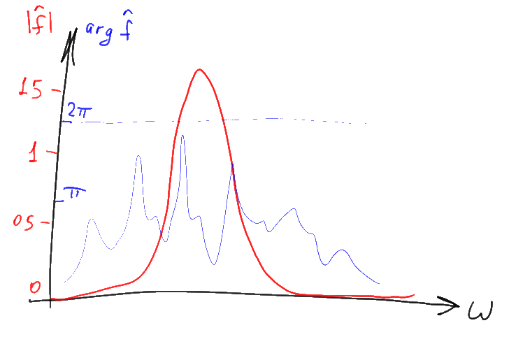
The graph of the complex value argument is often referred to as the “phase spectrum” in this case, and the modulus graph is often called the “amplitude spectrum”. The amplitude spectrum is usually of much greater interest, and therefore the “phase” part of the spectrum is often missed. In this article, we will also focus on “amplitude” things, but we should not forget about the existence of the missing phase part of the graph. In addition, instead of the usual module of the complex value, it is often drawn its log decimal multiplied by 10. As a result, a logarithmic graph is obtained, the values on which are displayed in decibels (dB).
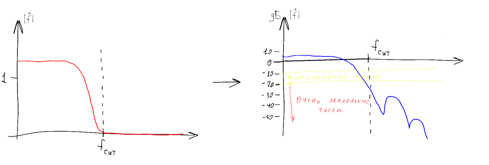
Note that not very much negative numbers of the logarithmic graph (-20 dB or less) correspond to almost zero numbers on the graph “normal”. Therefore, the long and wide “tails” of various spectra on such graphs, when mapped to “ordinary” coordinates, as a rule almost disappear. The convenience of this strange at first glance representation arises from the fact that the Fourier images of various functions often need to be multiplied together. With a similar pointwise multiplication of complex-valued Fourier transforms, their phase spectra are added, and the amplitude spectra are multiplied. The first is easy, and the second is relatively difficult. However, the amplitude logarithms when multiplied amplitudes are added, so logarithmic amplitude plots can, like the phase plots, just be added point-wise. In addition, in practical problems it is often more convenient to operate not with the “amplitude” of a signal, but with its “power” (square of amplitude). On a logarithmic scale, both graphs (and amplitudes and powers) look identical and differ only in coefficient — all values on the graph of power are exactly twice as large as on the scale of amplitudes. Accordingly, to build a graph of the distribution of power in frequency (in decibels), you can not build anything in a square, but calculate the decimal logarithm and multiply it by 20.
Are you bored? Wait a little more, with the boring part of the article explaining how to interpret the graphics, we'll be over soon :). But before that you should understand one extremely important thing: although all the above graphs of the spectra were drawn for some limited ranges of values (in particular, positive numbers), all of these graphs actually continue in plus and minus infinity. The graphs simply depict a certain “most informative” part of the graph, which is usually mirrored for negative parameter values and often repeats periodically with a certain step, if we consider it on a larger scale.
Having decided on what is drawn on the graphs, let's go back to the Fourier transform itself and its properties. There are several different ways to determine this transformation, differing in small details (different normalizations). For example, in our universities for some reason, the Fourier transform normalization is often used to determine the spectrum in terms of the angular frequency (radians per second). I will use a more convenient western formulation, defining the spectrum in terms of the usual frequency (hertz). The direct and inverse Fourier transforms in this case are determined by the formulas on the left, and some of the properties of this transformation that we need are a list of seven items on the right:
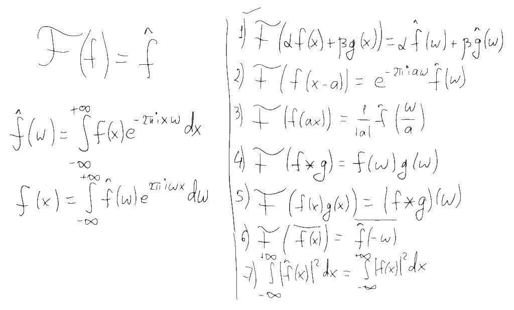
The first of these properties is linearity. If we take some kind of linear combination of functions, then the Fourier transform of this combination will be the same linear combination of Fourier images of these functions. This property allows us to reduce complex functions and their Fourier images to more simple ones. For example, the Fourier transform of a sinusoidal function with frequency f and amplitude a is a combination of two delta functions located at points f and -f and with a factor a / 2:

If we take a function consisting of the sum of a set of sinusoids with different frequencies, then according to the property of linearity, the Fourier transform of this function will consist of a corresponding set of delta functions. This allows us to give a naive but illustrative interpretation of the spectrum according to the principle “if in the spectrum of a function the frequency f corresponds to the amplitude a, then the original function can be represented as a sum of sinusoids, one of which will be a sinusoid with frequency f and amplitude 2a”. Strictly speaking, this interpretation is incorrect, since the delta function and the point on the graph are completely different things, but as we will see later, for discrete Fourier transforms it will not be so far from the truth.
The second property of the Fourier transform is the independence of the amplitude spectrum from the time shift of the signal. If we move the function to the left or right along the x axis, then only its phase spectrum will change.
The third property is the expansion (compression) of the original function along the time axis (x) proportionally compresses (stretches) its Fourier transform along the frequency scale (w). In particular, the spectrum of a signal of finite duration is always infinitely wide, and vice versa, a spectrum of finite width always corresponds to a signal of unlimited duration.
The fourth and fifth properties are probably the most useful of all. They allow us to reduce the convolution of functions to pointwise multiplication of their Fourier transforms and, conversely, the pointwise multiplication of functions to the convolution of their Fourier transforms. A little further, I will show how convenient it is.
The sixth property speaks of symmetry of Fourier transforms. In particular, it follows from this property that in a Fourier transform of a real-valued function (ie, any “real” signal), the amplitude spectrum is always an even function, and the phase spectrum (if it is brought to the range -pi ... pi) is odd . It is for this reason that the spectral plots almost never draw the negative part of the spectrum - for real-valued signals, it does not provide any new information (but, I repeat, it is not a zero one).
Finally, the last, seventh property, says that the Fourier transform conserves the “energy” of the signal. It is meaningful only for signals of finite duration, whose energy is finite, and suggests that the spectrum of such signals at infinity is rapidly approaching zero. It is because of this property that graphs of spectra usually represent only the “main” part of the signal, which carries the lion's share of energy - the rest of the graph simply goes to zero (but, again, is not zero).
Armed with these 7 properties, let's look at the math of “digitizing” a signal, which allows you to translate a continuous signal into a sequence of numbers. To do this, we need to take a function known as the “Dirac comb”:
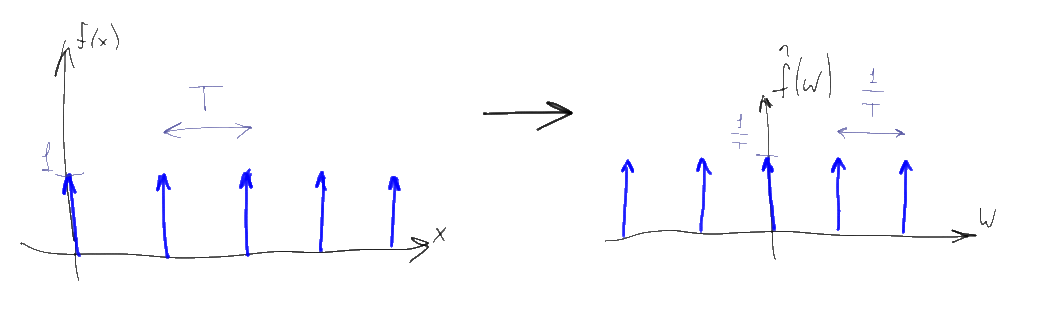
The Dirac comb is simply a periodic sequence of delta functions with a unit coefficient, starting at zero and going in increments of T. To digitize signals, T is chosen as small as possible, T << 1. The Fourier transform of this function is also a Dirac comb, only with a much larger 1 / T step and a slightly smaller coefficient (1 / T). From a mathematical point of view, the discretization of a signal over time is simply the pointwise multiplication of the original signal by a Dirac comb. The value of 1 / T is called the sampling rate:
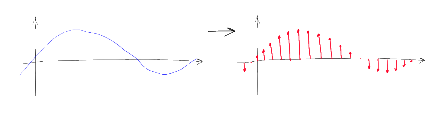
Instead of a continuous function after such a multiplication, a sequence of delta pulses of a certain height is obtained. Moreover, according to property 5 of the Fourier transform, the spectrum of the resulting discrete signal is a convolution of the original spectrum with the corresponding Dirac comb. It is easy to understand that, based on the properties of convolution, the spectrum of the original signal is “copied” infinitely many times along the frequency axis with a step of 1 / T, and then summed.
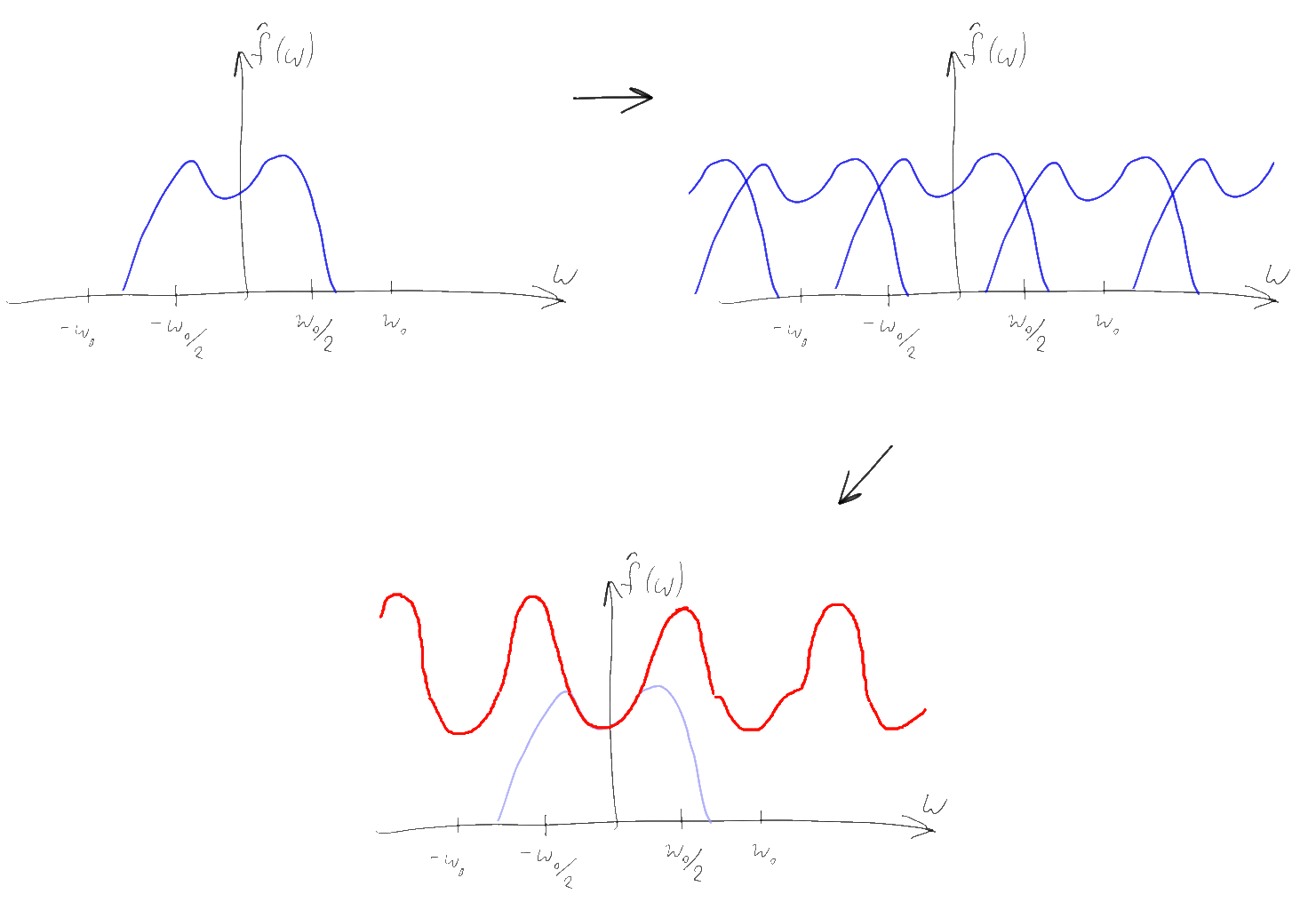
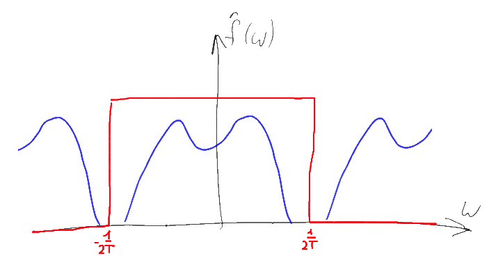
Note that if the original spectrum had a finite width and we used a sufficiently large sampling rate, then the copies of the original spectrum will not overlap, and therefore be added together. It is easy to understand that using such a “collapsed” spectrum it will be easy to restore the original one — it will be enough just to take the component of the spectrum near zero, “cutting off” the extra copies going to infinity. The simplest way to do this is to multiply the spectrum by a rectangular function equal to T in the range -1 / 2T ... 1 / 2T and zero — out of this range. Such a Fourier transform corresponds to the sinc (Tx) function and, according to property 4, this multiplication is equivalent to convolving the original sequence of delta functions with the sinc (Tx) function

That is, using the Fourier transform, we got a way to easily restore the original signal from the time sampled, operating under the condition that we use the sampling frequency, at least twice (due to the presence of negative frequencies in the spectrum) exceeding the maximum frequency present in the original signal. This result is widely known and is called the “Kotelnikov / Shannon-Nyquist theorem” . However, as it is easy now (understanding the proof) to notice, this result, contrary to widespread misconception, determines a sufficient but not necessary condition for the restoration of the original signal. All we need is to ensure that the part of the spectrum that we are interested in does not overlap each other after sampling the signal, and if the signal is narrow enough (has a small “width” of the non-zero part of the spectrum), then this result can often be achieved even at a sampling frequency than doubled the maximum signal frequency. Such a technique is called “undersampling” (sub-sampling, band-wise sampling ) and is quite widely used in the processing of various radio signals. For example, if we take FM radio operating in the frequency range from 88 to 108 MHz, then we can use the ADC with a frequency of only 43.5 MHz to digitize it instead of 216 MHz assumed by the Kotelnikov theorem. At the same time, however, you will need a high-quality ADC and a good filter.
I note that the “duplication” of high frequencies with frequencies of smaller orders (aliasing) is a direct property of signal sampling, an irreversible “spoiling” result. Therefore, if in the signal, in principle, high-order frequencies can be present (that is, almost always) an analog filter is put in front of the ADC, which “cuts off” everything superfluous directly in the original signal (since it will be too late to do this after sampling). The characteristics of these filters, as analog devices, are imperfect, so some “damage” of the signal still happens, and in practice it follows from this that the highest frequencies in the spectrum are usually unreliable. To reduce this problem, the signal is often sampled at an oversized sampling frequency, setting the input analog filter to a lower bandwidth and using only the lower part of the theoretically available frequency range of the ADC.
Another common misconception, by the way, is when the signal at the DAC output is drawn with “steps”. “Steps” correspond to the convolution of a discretized sequence of signals with a rectangular function of width T and height 1:
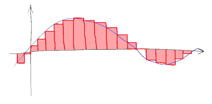
The signal spectrum in this transformation is multiplied by the Fourier transform of this rectangular function, and for a similar rectangular function this is again sinc (w), which is “stretched” the stronger, the smaller the width of the corresponding rectangle. The spectrum of the sampled signal with such a “DAC” is multiplied point by point by this spectrum. At the same time, unnecessary high frequencies with “extra copies” of the spectrum are not completely cut off, and the upper part of the “useful” part of the spectrum, on the contrary, is weakened.
In practice, of course, no one does. There are many different approaches to constructing a DAC, but even in the closest in the DAC weighing type, the rectangular pulses in the DAC, on the contrary, are selected as short as possible (approaching the current sequence of delta functions) to avoid excessive suppression of the useful part of the spectrum. The “extra” frequencies in the resulting broadband signal are almost always quenched by passing the signal through an analog low-pass filter, so that there are no “digital steps” either “inside” the converter or, especially, at its output.
But back to the Fourier transform. The Fourier transform described above applied to a pre-sampled signal sequence is called the Discrete Fourier Transform (DTFT). The spectrum obtained by such a transformation is always 1 / T-periodic, therefore the DTFT spectrum is completely determined by its values on the interval [0 ... 1 / T), therefore often the DTFT spectrum is often limited to this segment. At the same time, the result of DTFT, despite the fact that this is the spectrum of the sampled signal, is still an “analog” function. In addition, for “normal” valid-valued signals, the second half of this spectrum, by virtue of property 6, mirrors the left half, reflected from the Nyquist frequency 1 / 2T.
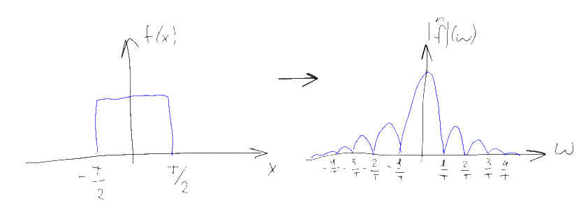
So far, we have assumed that the input of our transformations is a signal from minus to plus infinity. However, the real signals available to us always have a finite length - what to do? To solve this problem in FT and DTFT, the final signal is simply padded to the left and right to infinity with zeros. If the original signal was initially finite (say, a separate pulse) and it hit the Fourier transform completely, then this approach directly gives the desired result. However, often the “final” signal used for the Fourier transform is actually part of a longer, possibly infinite signal, such as a sinusoid, for example. In this case, the addition of the final segment with zeros is interpreted as follows: the initial signal is considered to be infinitely long, but then it is multiplied by some weighting function - the “window”, turning into zero beyond the segment available for us to measure. In the simplest case, the role of a “window” is simply a rectangular function, corresponding to the fact that we simply complement the final signal on the left and right with an infinite number of zeros. In more complex ones, the initial sequence is multiplied by weights determined by the “window” function and then, again, supplemented with zeros.
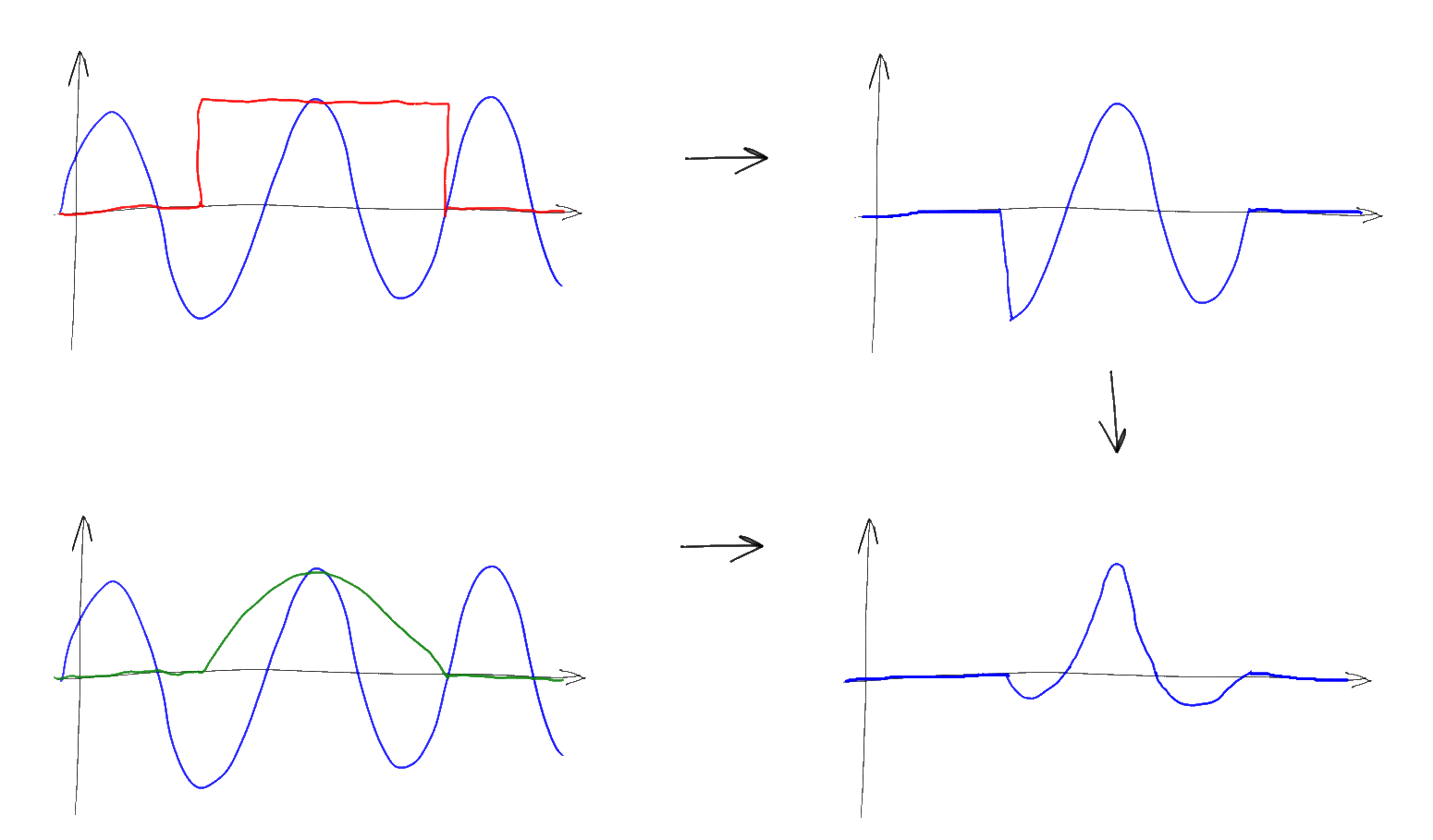
Using property 5, which is already familiar to us, it is easy to figure out that with such a multiplication, the original signal is simply minimized to the spectrum of the window function. For example, if we are trying to measure the spectrum of a sinusoid (the delta function), but limit the measurement interval to a rectangular window, then in the resulting spectrum in place of the delta function we will see the spectrum of the window - i.e. Tsinc (T (xf)):

In this case, T is the length of the interval by which we have limited our signal, so the longer the input signal is, the “narrower” and closer to the true delta function will be the spectrum we observe. The final “width” of the main lobe makes it impossible to confidently distinguish the presence of sinusoids in the original signal that are close to each other in frequency, and the presence of “side lobes” introduces small distortions into far-located frequencies, making it difficult to accurately measure the amplitude of individual frequencies, especially if you need to measure the spectrum in areas of small amplitude, if there are an order of magnitude more powerful components in the spectrum. This effect is called “spectral leakage” and it is impossible to completely defeat it for infinite signals, but the longer the interval at which the signal is measured, the less influence this leakage has. By choosing the window function, you can control the “width” of this leak, either by concentrating it around the main frequency (strongly “blurring” the spectrum, but not interfering with the neighboring frequencies), or spreading it everywhere (blurring of peaks decreases but the “noise” strongly increases and, as a result, error of measuring the amplitude of individual frequencies).Note that the selected sampling frequency in the spectral leakage almost does not matter - a short segment of the signal can be sampled at least 10 GHz, but this will increase only the number of measurable frequencies, while the accuracy of determining each individual frequency will still remain low.
An interesting particular case is the situation in which a signal with a set of discrete frequencies nF is discretized at a frequency mF, where m, n are integers. In this case, the zeros of the “window” and the arrangement of the delta functions in the spectrum coincide exactly and although the frequencies are still “smeared”, but their amplitude at the mF points coincides with the true one — the “noise” is zero. This property allows us to prove an analogue of Kotelnikov's theorem for the discrete Fourier transform, but in practice such signals, unfortunately, are not actually encountered.
So, with the “input” we figured out - from a continuous function of infinite length, we got a finite number of discrete samples that we can work with and instead received restrictions on the width of the spectrum and the leakage of frequencies. However, the “output” of the DTFT is still a continuous function, the work with which of the computer is problematic. In practice, this problem is solved very simply - the full segment [0.1 / T) is divided into k equal parts and DTFT is considered at the points fi = i / kT, where i = 0.1, ... k-1. The resulting construction is called the “Discrete Fourier Transform” (DFT).

It is convenient to normalize the last transformation by removing from it T and questions related to the choice of the “window”. This normalized notation is often used as the definition of a DFT as a transformation of a sequence of N complex numbers:

The beauty of the Fourier transform written in this form is that by retaining all the advantages of DTFT, like DTF for “smooth” k (for example, powers of two), it can be calculated extremely quickly, in a time of the order of k log (k). The corresponding algorithms are called the “fast Fourier transform” (FFT) and, generally speaking, there are several of them. From a practical point of view, however, all of them can be considered as “black boxes”, receiving a sequence of complex numbers at the input and issuing a sequence of complex numbers at the output. Thus, work with a finite-length discretized signal is reduced to the fact that this signal is first multiplied by a suitable weighing function, then supplemented with the necessary number of zeros to the right and transmitted to the FFT algorithm.
How to interpret the result? In view of the foregoing,
Well, in general, that's all. I hope the Fourier transform and FFT algorithms will now be for you simple, understandable and enjoyable tools.
(c) xkcdWithout using complex formulas and hardware, I will try to answer the following questions:
- FT, DTF, DTFT - what are the differences and how completely different seemingly formulas would give such conceptually similar results?
- How to interpret the results of the fast Fourier transform (FFT)
- What to do if a signal from 179 samples is given and the FFT requires a sequence of equal length of two at the input
- Why, when trying to get a spectrum of a sinusoid with the help of Fourier, instead of the expected single “stick”, a strange squiggle comes out on the graph and what can be done about it
- Why do analog filters are placed before the ADC and after the DAC?
- Is it possible to digitize the ADC signal with a frequency higher than half the sampling rate (the school answer is incorrect, the correct answer is possible)
- As the digital sequence restore the original signal
')
I will proceed from the assumption that the reader understands what an integral is , a complex number (as well as its module and argument ), convolution of functions , plus at least “on fingers” imagine what the Dirac delta function is . Do not know - it does not matter, read the above links. By “product of functions” in this text I will always understand “pointwise multiplication”
We must begin, probably, from the fact that the usual Fourier transform is some kind of thing that, as the name suggests, converts some functions to others, that is, assigns its spectrum or Fourier transform y to each function of a real variable x (t) (w):
If we give analogies, then an example of a transformation similar in meaning can be, for example, a differentiation that turns a function into its derivative. That is, the Fourier transform is the same, in essence, an operation as the taking of a derivative, and it is often denoted in a similar way, drawing a triangular “cap” over the function. But unlike differentiation, which can be defined for real numbers, the Fourier transform always “works” with more general complex numbers. Because of this, there are always problems with the display of the results of this transformation, since the complex numbers are determined not by one, but by two coordinates on a graph operating with real numbers. Most conveniently, as a rule, it turns out to present complex numbers as a module and argument and draw them separately as two separate graphs:
The graph of the complex value argument is often referred to as the “phase spectrum” in this case, and the modulus graph is often called the “amplitude spectrum”. The amplitude spectrum is usually of much greater interest, and therefore the “phase” part of the spectrum is often missed. In this article, we will also focus on “amplitude” things, but we should not forget about the existence of the missing phase part of the graph. In addition, instead of the usual module of the complex value, it is often drawn its log decimal multiplied by 10. As a result, a logarithmic graph is obtained, the values on which are displayed in decibels (dB).
Note that not very much negative numbers of the logarithmic graph (-20 dB or less) correspond to almost zero numbers on the graph “normal”. Therefore, the long and wide “tails” of various spectra on such graphs, when mapped to “ordinary” coordinates, as a rule almost disappear. The convenience of this strange at first glance representation arises from the fact that the Fourier images of various functions often need to be multiplied together. With a similar pointwise multiplication of complex-valued Fourier transforms, their phase spectra are added, and the amplitude spectra are multiplied. The first is easy, and the second is relatively difficult. However, the amplitude logarithms when multiplied amplitudes are added, so logarithmic amplitude plots can, like the phase plots, just be added point-wise. In addition, in practical problems it is often more convenient to operate not with the “amplitude” of a signal, but with its “power” (square of amplitude). On a logarithmic scale, both graphs (and amplitudes and powers) look identical and differ only in coefficient — all values on the graph of power are exactly twice as large as on the scale of amplitudes. Accordingly, to build a graph of the distribution of power in frequency (in decibels), you can not build anything in a square, but calculate the decimal logarithm and multiply it by 20.
Are you bored? Wait a little more, with the boring part of the article explaining how to interpret the graphics, we'll be over soon :). But before that you should understand one extremely important thing: although all the above graphs of the spectra were drawn for some limited ranges of values (in particular, positive numbers), all of these graphs actually continue in plus and minus infinity. The graphs simply depict a certain “most informative” part of the graph, which is usually mirrored for negative parameter values and often repeats periodically with a certain step, if we consider it on a larger scale.
Having decided on what is drawn on the graphs, let's go back to the Fourier transform itself and its properties. There are several different ways to determine this transformation, differing in small details (different normalizations). For example, in our universities for some reason, the Fourier transform normalization is often used to determine the spectrum in terms of the angular frequency (radians per second). I will use a more convenient western formulation, defining the spectrum in terms of the usual frequency (hertz). The direct and inverse Fourier transforms in this case are determined by the formulas on the left, and some of the properties of this transformation that we need are a list of seven items on the right:
The first of these properties is linearity. If we take some kind of linear combination of functions, then the Fourier transform of this combination will be the same linear combination of Fourier images of these functions. This property allows us to reduce complex functions and their Fourier images to more simple ones. For example, the Fourier transform of a sinusoidal function with frequency f and amplitude a is a combination of two delta functions located at points f and -f and with a factor a / 2:
If we take a function consisting of the sum of a set of sinusoids with different frequencies, then according to the property of linearity, the Fourier transform of this function will consist of a corresponding set of delta functions. This allows us to give a naive but illustrative interpretation of the spectrum according to the principle “if in the spectrum of a function the frequency f corresponds to the amplitude a, then the original function can be represented as a sum of sinusoids, one of which will be a sinusoid with frequency f and amplitude 2a”. Strictly speaking, this interpretation is incorrect, since the delta function and the point on the graph are completely different things, but as we will see later, for discrete Fourier transforms it will not be so far from the truth.
The second property of the Fourier transform is the independence of the amplitude spectrum from the time shift of the signal. If we move the function to the left or right along the x axis, then only its phase spectrum will change.
The third property is the expansion (compression) of the original function along the time axis (x) proportionally compresses (stretches) its Fourier transform along the frequency scale (w). In particular, the spectrum of a signal of finite duration is always infinitely wide, and vice versa, a spectrum of finite width always corresponds to a signal of unlimited duration.
The fourth and fifth properties are probably the most useful of all. They allow us to reduce the convolution of functions to pointwise multiplication of their Fourier transforms and, conversely, the pointwise multiplication of functions to the convolution of their Fourier transforms. A little further, I will show how convenient it is.
The sixth property speaks of symmetry of Fourier transforms. In particular, it follows from this property that in a Fourier transform of a real-valued function (ie, any “real” signal), the amplitude spectrum is always an even function, and the phase spectrum (if it is brought to the range -pi ... pi) is odd . It is for this reason that the spectral plots almost never draw the negative part of the spectrum - for real-valued signals, it does not provide any new information (but, I repeat, it is not a zero one).
Finally, the last, seventh property, says that the Fourier transform conserves the “energy” of the signal. It is meaningful only for signals of finite duration, whose energy is finite, and suggests that the spectrum of such signals at infinity is rapidly approaching zero. It is because of this property that graphs of spectra usually represent only the “main” part of the signal, which carries the lion's share of energy - the rest of the graph simply goes to zero (but, again, is not zero).
Armed with these 7 properties, let's look at the math of “digitizing” a signal, which allows you to translate a continuous signal into a sequence of numbers. To do this, we need to take a function known as the “Dirac comb”:
The Dirac comb is simply a periodic sequence of delta functions with a unit coefficient, starting at zero and going in increments of T. To digitize signals, T is chosen as small as possible, T << 1. The Fourier transform of this function is also a Dirac comb, only with a much larger 1 / T step and a slightly smaller coefficient (1 / T). From a mathematical point of view, the discretization of a signal over time is simply the pointwise multiplication of the original signal by a Dirac comb. The value of 1 / T is called the sampling rate:
Instead of a continuous function after such a multiplication, a sequence of delta pulses of a certain height is obtained. Moreover, according to property 5 of the Fourier transform, the spectrum of the resulting discrete signal is a convolution of the original spectrum with the corresponding Dirac comb. It is easy to understand that, based on the properties of convolution, the spectrum of the original signal is “copied” infinitely many times along the frequency axis with a step of 1 / T, and then summed.
Note that if the original spectrum had a finite width and we used a sufficiently large sampling rate, then the copies of the original spectrum will not overlap, and therefore be added together. It is easy to understand that using such a “collapsed” spectrum it will be easy to restore the original one — it will be enough just to take the component of the spectrum near zero, “cutting off” the extra copies going to infinity. The simplest way to do this is to multiply the spectrum by a rectangular function equal to T in the range -1 / 2T ... 1 / 2T and zero — out of this range. Such a Fourier transform corresponds to the sinc (Tx) function and, according to property 4, this multiplication is equivalent to convolving the original sequence of delta functions with the sinc (Tx) function
That is, using the Fourier transform, we got a way to easily restore the original signal from the time sampled, operating under the condition that we use the sampling frequency, at least twice (due to the presence of negative frequencies in the spectrum) exceeding the maximum frequency present in the original signal. This result is widely known and is called the “Kotelnikov / Shannon-Nyquist theorem” . However, as it is easy now (understanding the proof) to notice, this result, contrary to widespread misconception, determines a sufficient but not necessary condition for the restoration of the original signal. All we need is to ensure that the part of the spectrum that we are interested in does not overlap each other after sampling the signal, and if the signal is narrow enough (has a small “width” of the non-zero part of the spectrum), then this result can often be achieved even at a sampling frequency than doubled the maximum signal frequency. Such a technique is called “undersampling” (sub-sampling, band-wise sampling ) and is quite widely used in the processing of various radio signals. For example, if we take FM radio operating in the frequency range from 88 to 108 MHz, then we can use the ADC with a frequency of only 43.5 MHz to digitize it instead of 216 MHz assumed by the Kotelnikov theorem. At the same time, however, you will need a high-quality ADC and a good filter.
I note that the “duplication” of high frequencies with frequencies of smaller orders (aliasing) is a direct property of signal sampling, an irreversible “spoiling” result. Therefore, if in the signal, in principle, high-order frequencies can be present (that is, almost always) an analog filter is put in front of the ADC, which “cuts off” everything superfluous directly in the original signal (since it will be too late to do this after sampling). The characteristics of these filters, as analog devices, are imperfect, so some “damage” of the signal still happens, and in practice it follows from this that the highest frequencies in the spectrum are usually unreliable. To reduce this problem, the signal is often sampled at an oversized sampling frequency, setting the input analog filter to a lower bandwidth and using only the lower part of the theoretically available frequency range of the ADC.
Another common misconception, by the way, is when the signal at the DAC output is drawn with “steps”. “Steps” correspond to the convolution of a discretized sequence of signals with a rectangular function of width T and height 1:
The signal spectrum in this transformation is multiplied by the Fourier transform of this rectangular function, and for a similar rectangular function this is again sinc (w), which is “stretched” the stronger, the smaller the width of the corresponding rectangle. The spectrum of the sampled signal with such a “DAC” is multiplied point by point by this spectrum. At the same time, unnecessary high frequencies with “extra copies” of the spectrum are not completely cut off, and the upper part of the “useful” part of the spectrum, on the contrary, is weakened.
In practice, of course, no one does. There are many different approaches to constructing a DAC, but even in the closest in the DAC weighing type, the rectangular pulses in the DAC, on the contrary, are selected as short as possible (approaching the current sequence of delta functions) to avoid excessive suppression of the useful part of the spectrum. The “extra” frequencies in the resulting broadband signal are almost always quenched by passing the signal through an analog low-pass filter, so that there are no “digital steps” either “inside” the converter or, especially, at its output.
But back to the Fourier transform. The Fourier transform described above applied to a pre-sampled signal sequence is called the Discrete Fourier Transform (DTFT). The spectrum obtained by such a transformation is always 1 / T-periodic, therefore the DTFT spectrum is completely determined by its values on the interval [0 ... 1 / T), therefore often the DTFT spectrum is often limited to this segment. At the same time, the result of DTFT, despite the fact that this is the spectrum of the sampled signal, is still an “analog” function. In addition, for “normal” valid-valued signals, the second half of this spectrum, by virtue of property 6, mirrors the left half, reflected from the Nyquist frequency 1 / 2T.
So far, we have assumed that the input of our transformations is a signal from minus to plus infinity. However, the real signals available to us always have a finite length - what to do? To solve this problem in FT and DTFT, the final signal is simply padded to the left and right to infinity with zeros. If the original signal was initially finite (say, a separate pulse) and it hit the Fourier transform completely, then this approach directly gives the desired result. However, often the “final” signal used for the Fourier transform is actually part of a longer, possibly infinite signal, such as a sinusoid, for example. In this case, the addition of the final segment with zeros is interpreted as follows: the initial signal is considered to be infinitely long, but then it is multiplied by some weighting function - the “window”, turning into zero beyond the segment available for us to measure. In the simplest case, the role of a “window” is simply a rectangular function, corresponding to the fact that we simply complement the final signal on the left and right with an infinite number of zeros. In more complex ones, the initial sequence is multiplied by weights determined by the “window” function and then, again, supplemented with zeros.
Using property 5, which is already familiar to us, it is easy to figure out that with such a multiplication, the original signal is simply minimized to the spectrum of the window function. For example, if we are trying to measure the spectrum of a sinusoid (the delta function), but limit the measurement interval to a rectangular window, then in the resulting spectrum in place of the delta function we will see the spectrum of the window - i.e. Tsinc (T (xf)):
In this case, T is the length of the interval by which we have limited our signal, so the longer the input signal is, the “narrower” and closer to the true delta function will be the spectrum we observe. The final “width” of the main lobe makes it impossible to confidently distinguish the presence of sinusoids in the original signal that are close to each other in frequency, and the presence of “side lobes” introduces small distortions into far-located frequencies, making it difficult to accurately measure the amplitude of individual frequencies, especially if you need to measure the spectrum in areas of small amplitude, if there are an order of magnitude more powerful components in the spectrum. This effect is called “spectral leakage” and it is impossible to completely defeat it for infinite signals, but the longer the interval at which the signal is measured, the less influence this leakage has. By choosing the window function, you can control the “width” of this leak, either by concentrating it around the main frequency (strongly “blurring” the spectrum, but not interfering with the neighboring frequencies), or spreading it everywhere (blurring of peaks decreases but the “noise” strongly increases and, as a result, error of measuring the amplitude of individual frequencies).Note that the selected sampling frequency in the spectral leakage almost does not matter - a short segment of the signal can be sampled at least 10 GHz, but this will increase only the number of measurable frequencies, while the accuracy of determining each individual frequency will still remain low.
An interesting particular case is the situation in which a signal with a set of discrete frequencies nF is discretized at a frequency mF, where m, n are integers. In this case, the zeros of the “window” and the arrangement of the delta functions in the spectrum coincide exactly and although the frequencies are still “smeared”, but their amplitude at the mF points coincides with the true one — the “noise” is zero. This property allows us to prove an analogue of Kotelnikov's theorem for the discrete Fourier transform, but in practice such signals, unfortunately, are not actually encountered.
So, with the “input” we figured out - from a continuous function of infinite length, we got a finite number of discrete samples that we can work with and instead received restrictions on the width of the spectrum and the leakage of frequencies. However, the “output” of the DTFT is still a continuous function, the work with which of the computer is problematic. In practice, this problem is solved very simply - the full segment [0.1 / T) is divided into k equal parts and DTFT is considered at the points fi = i / kT, where i = 0.1, ... k-1. The resulting construction is called the “Discrete Fourier Transform” (DFT).
It is convenient to normalize the last transformation by removing from it T and questions related to the choice of the “window”. This normalized notation is often used as the definition of a DFT as a transformation of a sequence of N complex numbers:
The beauty of the Fourier transform written in this form is that by retaining all the advantages of DTFT, like DTF for “smooth” k (for example, powers of two), it can be calculated extremely quickly, in a time of the order of k log (k). The corresponding algorithms are called the “fast Fourier transform” (FFT) and, generally speaking, there are several of them. From a practical point of view, however, all of them can be considered as “black boxes”, receiving a sequence of complex numbers at the input and issuing a sequence of complex numbers at the output. Thus, work with a finite-length discretized signal is reduced to the fact that this signal is first multiplied by a suitable weighing function, then supplemented with the necessary number of zeros to the right and transmitted to the FFT algorithm.
How to interpret the result? In view of the foregoing,
- The resulting values are a uniform grid of samples across the DTFT spectrum. The more readings - the finer the grid, the more visible the spectrum. By adding the required number of zeros to a known sequence, one can calculate an arbitrarily close approximation to the continuous spectrum.
- The DTFT spectrum is specified on a frequency interval from 0 to 1 / T (where 1 / T is the sampling frequency) and periodically repeats to infinity outside this segment
- This spectrum is given by complex numbers (pairs of real). The amplitude is defined as the modulus of a complex number, the phase as an argument.
- For a valid input signal, the spectrum in the range 1 / 2T ... 1 / T simply mirrors the spectrum 0 ... 1 / 2T and does not carry the payload (for visualizing the spectrum, you can simply cut it off)
- , ( ) —
- “ ” “ ”. ( !) — .
- . , , , , k/T.
- A ( ) A*N/2, , “” “” A*N, 1/2T ( A*N, , ). N = T1/T0, T1 — ( «»), T0 — ( ) , , ( )
Well, in general, that's all. I hope the Fourier transform and FFT algorithms will now be for you simple, understandable and enjoyable tools.
Source: https://habr.com/ru/post/196374/
All Articles