Numenta NuPIC: First Steps

Introduction

Numenta NuPIC is an open implementation of algorithms that simulate the processes of storing information by a person, occurring in the neocortex. NuPIC source codes on github

In a nutshell, the purpose of NuPIC can be described as "figovina, identifying, memorizing and predicting spatial and temporal patterns in the data." The human brain deals with this most of the time - it remembers, summarizes and predicts. A very good description of these processes can be found in Jeff Hawkins's On Intelligence book (there is a Russian translation of the book titled On Intellect).

On the Numenta website there is a detailed document detailing the algorithms and principles of operation, as well as several videos.
')

Assembly and installation

Described in the readme file in the repository, so I will not detail. To work, nupic will require python2.7 (or 2.6) with header files.

Model parameters and structure

The key concept of nupic is the neocortex model (or simply the model), which is a collection of cells that process and store input data. In the process of processing the input data, the cells predict the likely development of events, which automatically generates a forecast for the future. About how this is done, I will tell in the next article, now only a general description of the most necessary things.

The model consists of several processes, the behavior of each of which is defined by a set of parameters.

Encoder

The input data passes through the encoder, transforming into a clear view of the model. Each cell perceives only binary data, and for work, data close in meaning should have a similar binary representation.

For example, we want to input numbers from the range from 1 to 100 (say, the current relative humidity) to the input of the model. If you just take the binary representation of the numbers, that the values ​​7 and 8, are located side by side, but their binary representation differs very much (0b0111 and 0b1000). To avoid this, the encoder converts numeric values ​​to a set of one bits, shifted in proportion to the value. For example, for a range of values ​​from 1 to 10 and three unit bits, we get the following representation:

• 1 -> 11.1 billion
• 2 -> 011100000000
• 3 -> 001110000000
• 7 -> 000000111000
• 10 -> 000000000111

If multiple values ​​are input, their binary representations are simply merged together.
Similarly, floating-point and discrete values ​​(true / false, and other enumerated types) are represented.

Spatial pooler

The main objective of SP is to ensure the activation of a close set of cells to a similar data set, adding an element of randomness to this activation. A detailed discussion of how this is done is beyond the scope of the article. Those interested can wait to continue, or refer to the original whitepaper.

Temporal pooler

In addition to identifying similar images of input data, NuPIC can distinguish the context of this data by analyzing their flow over time. This is achieved through the layering of a set of cells (the so-called cell columns), and a detailed description also goes beyond the intended limits. It suffices to say that without this, the system would not distinguish the character B in the sequence ABCABC from the same character in the CBACBA.

Practice: sine

Enough theory, move on to the practical side of the issue. To begin with, let's take a simple sine function, feed the model input and see how well it can understand and predict it.

Full code example , analyze key points.

To create a model based on a set of parameters, the ModelFactory class is used:

from nupic.frameworks.opf.modelfactory import ModelFactory model = ModelFactory.create(model_params.MODEL_PARAMS) model.enableInference({'predictedField': 'y'}) 

MODEL_PARAMS is a rather spreading dict with a full set of model parameters. All the parameters we are not interested in now, but on some it will stop.

  'sensorParams': { 'encoders': { 'y': { 'fieldname': u'y', 'n': 100, 'name': u'y', 'type': 'ScalarEncoder', 'minval': -1.0, 'maxval': 1.0, 'w': 21 }, }, 

Here, the parameters of the encodera are set, which converts the sine value (in the range from -1 to 1) into a bit representation. The values ​​minval and maxval determine the range, the value n sets the total number of bits in the result, and w the number of single bits (for some reason it must be odd). Thus, the entire range is divided into 79 intervals in increments of 0.025. For verification is enough.

The remaining parameters do not need to be changed yet - there are many of them, but the default values ​​work fine. Even after reading the witepaper and several months of digging with the code, the exact purpose of some of the options remains a mystery to me.

Calling the enableInference method on the model indicates which of the input parameters we want to predict (there can be only one).

Preparation is completed, you can pump the model data. This is done like this:

 res = model.run({'y': y}) 

The arguments are given a dict, which lists all input values. At the output, the model returns an object containing a copy of the input data (both in the original representation and in the encoded one), as well as a forecast for the next step. Most of all we are interested in the forecast in the field inferences:

 {'encodings': [array([ 0., 0., 0., 0., 0., 0., 0., 0., 0., 0., 0., 0., 0., 0., 0., 0., 0., 0., 0., 0., 0., 0., 0., 0., 0., 0., 0., 0., 0., 0., 0., 0., 0., 0., 0., 0., 0., 0., 0., 0., 0., 0., 0., 0., 0., 0., 0., 0., 0., 0., 0., 0., 0., 0., 0., 0., 0., 0., 0., 1., 1., 1., 1., 1., 1., 1., 0., 0., 0., 0., 0., 0., 0., 0., 0., 0., 0., 0., 0., 0., 0., 0., 0., 0., 0., 0., 0., 0., 0., 0., 0., 0., 0., 0., 0., 0., 0., 0., 0., 0.], dtype=float32)], 'multiStepBestPredictions': {1: 0.2638645383168643}, 'multiStepPredictions': {1: {0.17879642297981466: 0.0083312500347378464, 0.20791169081775931: 0.0083320832430621525, 0.224951054343865: 0.020831041503470333, 0.24192189559966773: 0.054163124704840825, 0.2638645383168643: 0.90834250051388887}}, 

We can predict several steps at once, so in the multiStepPredictions dictionary, the key is the number of prediction steps, and the value is another dictionary with a prediction in the key and a probability in the value. For the example above, the model predicts a value of 0.26386 with a probability of 90.83%, a value of 0.2419 with a probability of 5.4%, etc.

The most likely prediction is in the multiStepBestPredictions field.

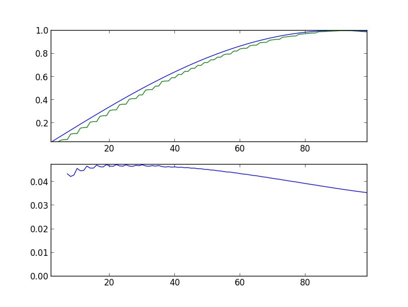
Armed with all this knowledge, we are trying to predict a simple sine. Below are the graphs of the program runs, with the indication of the launch parameters. In the upper graph, the blue line is the original sine, the green line is the model's forecast, shifted one step to the left. In the lower graph, the root mean square error is 360 values ​​back (full period).

Initially, the error is quite large, and the predicted value differs markedly from the original value (sin-predictor.py -s 100):


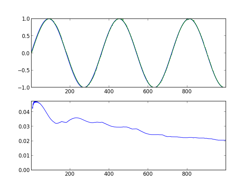
After 1000 steps:


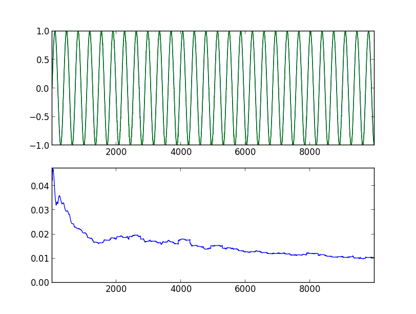
Progress is evident. After 10,000 steps:


After 10,000 steps, the last 360 values:


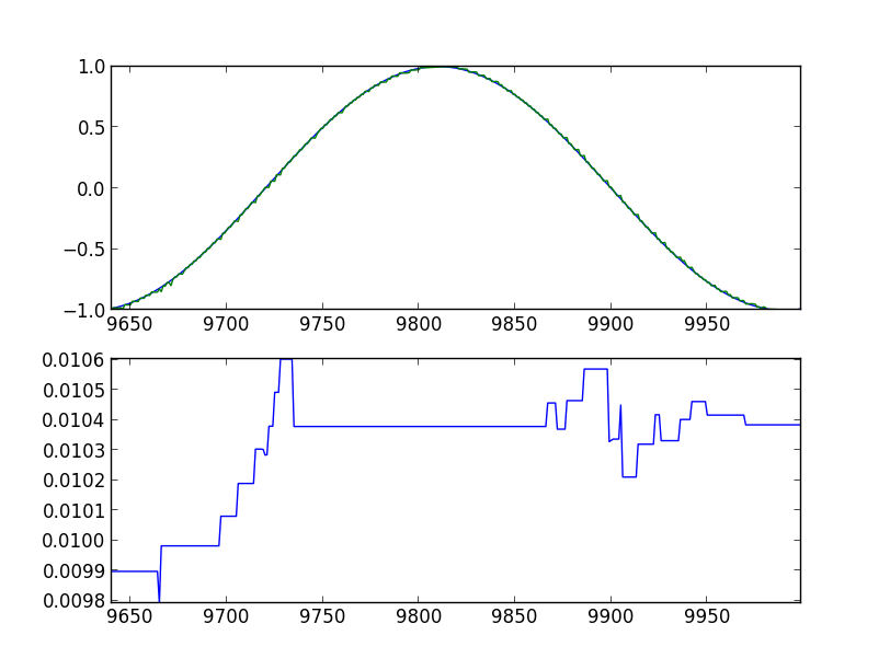
It can be seen that the model definitely got some ideas about what they want from it.

Conclusion

In this article I tried to give the most general idea of ​​how to use NuPIC, without going into the jungle of implementation details. Behind the scenes, there are a lot of things - network structure, cerebro visualization system, swarming, etc. If there is time and interest in the topic, the article can be continued.