Introduction to the analysis of the complexity of algorithms (part 3)
From the translator: this text is given with insignificant abbreviations due to places of excessive “razvezhnannosti” material. The author absolutely rightly warns that certain topics may seem too simple or well-known to the reader. Nevertheless, personally this text helped me to streamline the existing knowledge on the analysis of the complexity of algorithms. I hope that it will be useful to someone else.
Due to the large volume of the original article, I broke it into pieces, which in total will be four.
I (as always) would be extremely grateful for any comments in PM about improving the quality of the translation.
Published previously:
Part 1
Part 2
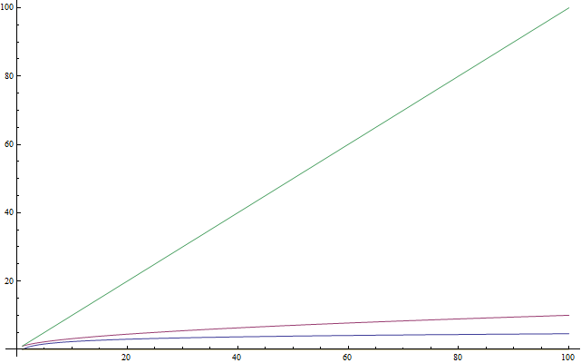
If you know what logarithms are, you can safely skip this section. The chapter is intended for those who are unfamiliar with this concept or use it so rarely that they have already forgotten what it is all about. Logarithms are important because they are very often found when analyzing complexity. Logarithm is an operation that, when applied to a number, makes it much smaller (like taking a square root). So the first thing you need to remember: a logarithm returns a number less than the original. In the figure on the right, the green graph is the linear function
Let me explain by example. Consider the equation
')
To find
Practical recommendation: at competitions algorithms are often implemented in C ++. Once you have analyzed the complexity of your algorithm, you can immediately get a rough estimate of how quickly it will work, assuming that 1,000,000 commands are executed per second. Their number is calculated from the asymptotic estimate function obtained by you, which describes the algorithm. For example, the calculation using the algorithm with Θ (n) takes about a second with n = 1,000,000.
Now let's turn to recursive functions. A recursive function is a function that calls itself. Can we analyze its complexity? The following function, written in Python, calculates the factorial of a given number. The factorial of a positive integer is found as the product of all previous positive integers. For example, factorial 5 is
Let's analyze this function. It does not contain cycles, but its complexity is still not constant. Well, you have to re-start counting instructions. Obviously, if we apply this function to some
If you are still not sure of this, then you can always find the exact complexity by counting the number of instructions. Apply this method to this function to find its f (n), and make sure that it is linear (recall that linearity means
One of the most famous tasks in computer science is to search for values in an array. We have already solved it for the general case. The task becomes more interesting if we have a sorted array in which we want to find the specified value. One way to do this is binary search . We take the middle element from our array: if it matches what we were looking for, then the problem is solved. Otherwise, if the specified value is greater than this element, then we know that it must lie on the right side of the array. And if less - then on the left. We will split these subarrays until we get what we want.
Here is the implementation of such a method in pseudocode:
The above pseudo-code simplifies the present implementation. In practice, this method is easier to describe than to implement, because the programmer needs to solve some additional issues. For example, error protection by one position ( off-by-one error, OBOE ), and even dividing by two may not always give an integer, so you will need to use the
If you are not sure that the method works in principle, then get distracted and decide manually some simple example.
Now let's try to analyze this algorithm. Once again, in this case we have a recursive algorithm. Let's assume for simplicity that the array is always split exactly in half, ignoring the +1 and -1 parts in a recursive call. At this point, you should be sure that such a small change as ignoring +1 and -1 will not affect the final result of the complexity assessment. In principle, this fact is usually necessary to prove if we want to be careful from a mathematical point of view. But in practice it is obvious at the level of intuition. Also for simplicity, let's assume that our array is the size of one of the powers of two. Again, this assumption will in no way affect the final result of the calculation of the complexity of the algorithm. The worst scenario for this task would be the option when the array in principle does not contain the desired value. In this case, we start with an array of size
0th iteration:
1st iteration:
2nd iteration:
3rd iteration:
...
i-th iteration:
...
last iteration:
Note that at the ith iteration, the array has
Equality will be true only when we reach the final call to the
If you read the section on logarithms above, then this expression will be familiar to you. Solving it, we get:
This answer tells us that the number of iterations required for a binary search is
If you think a little, it makes sense. For example, take
The latter result allows us to compare binary search with a linear (our previous method). Undoubtedly,
Practical recommendation: improving the asymptotic runtime of a program often greatly improves its performance. Much stronger than a small "technical" optimization in the form of using a faster programming language.
Due to the large volume of the original article, I broke it into pieces, which in total will be four.
I (as always) would be extremely grateful for any comments in PM about improving the quality of the translation.
Published previously:
Part 1
Part 2
Logarithms
If you know what logarithms are, you can safely skip this section. The chapter is intended for those who are unfamiliar with this concept or use it so rarely that they have already forgotten what it is all about. Logarithms are important because they are very often found when analyzing complexity. Logarithm is an operation that, when applied to a number, makes it much smaller (like taking a square root). So the first thing you need to remember: a logarithm returns a number less than the original. In the figure on the right, the green graph is the linear function
f(n) = n , the red one is f(n) = sqrt(n) , and the least rapidly increasing one is f(n) = log(n) . Next: just as taking a square root is the inverse operation of squaring, logarithm is the inverse operation of raising something to a power.Let me explain by example. Consider the equation
')
2 x = 1024To find
x from it, we ask ourselves: to what degree should we build 2 to get 1024? Answer: the tenth. In fact, 2 10 = 1024 , which is easy to check. Logarithms help us describe this problem using a new notation. In this case, 10 is the logarithm of 1024 and is written as log (1024). Read: "logarithm 1024". Since we used 2 as the base, such logarithms are called “base 2”. The base can be any number, but in this article we will use only two. If you are an academic student and are not familiar with logarithms, then I recommend you practice after you finish reading this article. In computer science, logarithms on base 2 are more common than any others, because often we have only two entities: 0 and 1. There is also a tendency to split volume tasks in half, and the halves, as is well known, are also only two. Therefore, for further reading of the article, you only need to have an idea about the logarithms of base 2.Exercise 7
Solve the equations below by writing the logarithms you are looking for. Use only base 2 logarithms.
- 2 x = 64
- (2 2 ) x = 64
- 4 x = 4
- 2 x = 1
- 2 x + 2 x = 32
- (2 x) * (2 x ) = 64
Decision
It does not need anything beyond the ideas outlined above.
- By trial and error, we find that
x = 6. Thus,log( 64 ) = 6 - By the property of degrees (2 2 ) x can be written as 2 2 x . Thus, we obtain
2x = 6(becauselog( 64 ) = 6from the previous example) and, therefore,x = 3 - Using the knowledge gained from solving the previous example, we write 4 as 2 2 . Then our equation turns into (2 2 ) x = 4, which is equivalent to 2 2 x . Note that log (4) = 2 (since 2 2 = 4), so we get
2x = 2, hencex = 1. This is easily noticed by the original equation, since a power of 1 gives a basis as a result. - Recalling that degree 0 gives the result 1 (i.e.
log( 1 ) = 0), we getx = 0 - Here we are dealing with a sum, so it’s impossible to directly take the logarithm. However, we notice that
2x+ 2x is the same as2 * (2x). Multiplying by 2 gives2x + 1 , and we get the equation2x + 1= 32. We find thatlog( 32 ) = 5, whencex + 1 = 5andx = 4. - We multiply two powers of two, therefore, we can combine them in 2 2x . It remains only to solve the equation
22x= 64, which we have already done above. Answer:x = 3
Practical recommendation: at competitions algorithms are often implemented in C ++. Once you have analyzed the complexity of your algorithm, you can immediately get a rough estimate of how quickly it will work, assuming that 1,000,000 commands are executed per second. Their number is calculated from the asymptotic estimate function obtained by you, which describes the algorithm. For example, the calculation using the algorithm with Θ (n) takes about a second with n = 1,000,000.
Recursive complexity
Now let's turn to recursive functions. A recursive function is a function that calls itself. Can we analyze its complexity? The following function, written in Python, calculates the factorial of a given number. The factorial of a positive integer is found as the product of all previous positive integers. For example, factorial 5 is
5 * 4 * 3 * 2 * 1 . It is designated as “5!” And pronounced “factorial five” (however, some prefer “FIVE !!! 11”). def factorial( n ): if n == 1: return 1 return n * factorial( n - 1 ) Let's analyze this function. It does not contain cycles, but its complexity is still not constant. Well, you have to re-start counting instructions. Obviously, if we apply this function to some
n , then it will be calculated n times. (If you are not sure about this, you can manually write the calculation flow with n = 5 to determine how this actually works.) Thus, we see that this function is Θ( n ) .If you are still not sure of this, then you can always find the exact complexity by counting the number of instructions. Apply this method to this function to find its f (n), and make sure that it is linear (recall that linearity means
Θ( n ) ).Logarithmic complexity
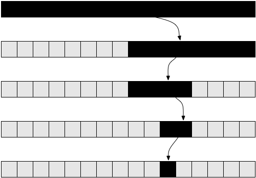
One of the most famous tasks in computer science is to search for values in an array. We have already solved it for the general case. The task becomes more interesting if we have a sorted array in which we want to find the specified value. One way to do this is binary search . We take the middle element from our array: if it matches what we were looking for, then the problem is solved. Otherwise, if the specified value is greater than this element, then we know that it must lie on the right side of the array. And if less - then on the left. We will split these subarrays until we get what we want.
Here is the implementation of such a method in pseudocode:
def binarySearch( A, n, value ): if n = 1: if A[ 0 ] = value: return true else: return false if value < A[ n / 2 ]: return binarySearch( A[ 0...( n / 2 - 1 ) ], n / 2 - 1, value ) else if value > A[ n / 2 ]: return binarySearch( A[ ( n / 2 + 1 )...n ], n / 2 - 1, value ) else: return true The above pseudo-code simplifies the present implementation. In practice, this method is easier to describe than to implement, because the programmer needs to solve some additional issues. For example, error protection by one position ( off-by-one error, OBOE ), and even dividing by two may not always give an integer, so you will need to use the
floor() or ceil() functions. However, suppose that in our case the division will always be successful, our code is protected from off-by-one errors, and all we want is to analyze the complexity of this method. If you have never implemented a binary search, you can do it in your favorite programming language. Such a task is truly instructive.If you are not sure that the method works in principle, then get distracted and decide manually some simple example.
Now let's try to analyze this algorithm. Once again, in this case we have a recursive algorithm. Let's assume for simplicity that the array is always split exactly in half, ignoring the +1 and -1 parts in a recursive call. At this point, you should be sure that such a small change as ignoring +1 and -1 will not affect the final result of the complexity assessment. In principle, this fact is usually necessary to prove if we want to be careful from a mathematical point of view. But in practice it is obvious at the level of intuition. Also for simplicity, let's assume that our array is the size of one of the powers of two. Again, this assumption will in no way affect the final result of the calculation of the complexity of the algorithm. The worst scenario for this task would be the option when the array in principle does not contain the desired value. In this case, we start with an array of size
n on the first recursive call, n / 2 on the second, n / 4 on the third, and so on. In general, our array is split in half on each call until we reach one. Let's write the number of elements in the array on each call:0th iteration:
n1st iteration:
n / 22nd iteration:
n / 43rd iteration:
n / 8...
i-th iteration:
n / 2 i...
last iteration:
1Note that at the ith iteration, the array has
n / 2 i elements. We split it in half each time, which means dividing the number of elements by two (equivalent to multiplying the denominator by two). Having done this i times, we get n / 2 i . The process will continue, and from each large i we will receive a smaller number of elements until we reach one. If we want to know at what iteration this happened, we will just need to solve the following equation:1 = n / 2 iEquality will be true only when we reach the final call to the
binarySearch() function, so by learning i from it, we will know the number of the last recursive iteration. Multiplying both sides by 2 i , we get:2 i = nIf you read the section on logarithms above, then this expression will be familiar to you. Solving it, we get:
i = log( n )This answer tells us that the number of iterations required for a binary search is
log( n ) , where n is the size of the original array.If you think a little, it makes sense. For example, take
n = 32 (an array of 32 elements). How many times will we need to split it to get one item? We count: 32 → 16 → 8 → 4 → 2 → 1 - a total of 5 times, which is the logarithm of 32. Thus, the complexity of the binary search is Θ( log( n ) ) .The latter result allows us to compare binary search with a linear (our previous method). Undoubtedly,
log( n ) much smaller than n , from which it is legitimate to conclude that the former is much faster than the latter. So it makes sense to store arrays in a sorted form, if we are going to look for values in them often.Practical recommendation: improving the asymptotic runtime of a program often greatly improves its performance. Much stronger than a small "technical" optimization in the form of using a faster programming language.
Source: https://habr.com/ru/post/195996/
All Articles