Evaluation of linear regression results

Introduction

Today, everyone who is even slightly interested in mining is probably heard about a simple linear regression . About it already wrote on Habré, as well as told in detail about Andrew Ng in his famous machine learning course. Linear regression is one of the basic and simplest methods of machine learning, however, methods for assessing the quality of the constructed model are rarely mentioned. In this article I will try to correct this annoying omission a little by examining the results of the function summary.lm () in the R language. At the same time, I will try to provide the necessary formulas so that all calculations can be easily programmed in any other language. This article is intended for those who have heard that it is possible to construct a linear regression, but have not encountered statistical procedures to assess its quality.

Linear regression model

So, let there be several independent random variables X1, X2, ..., Xn (predictors) and the quantity Y depending on them (it is assumed that all the necessary predictor transformations have already been made). Moreover, we assume that the dependence is linear, and the errors are normally distributed, that is,

where I is the unit square matrix of size nx n.

So, we have data consisting of k observations of Y and Xi values ​​and we want to estimate the coefficients. The standard method for finding estimates of coefficients is the method of least squares . And the analytical solution that can be obtained by applying this method looks like this:

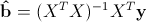
where b with a lid is an estimate of the coefficient vector, y is a vector of values ​​of the dependent variable, and X is a matrix of size kx n + 1 (n is the number of predictors, k is the number of observations), in which the first column consists of ones, the second is the value of the first predictor , the third - the second and so on, and the lines correspond to the available observations.

Function summary.lm () and evaluation of the results

Now consider an example of building a linear regression model in the language R:

> library(faraway) > lm1<-lm(Species~Area+Elevation+Nearest+Scruz+Adjacent, data=gala) > summary(lm1) Call: lm(formula = Species ~ Area + Elevation + Nearest + Scruz + Adjacent, data = gala) Residuals: Min 1Q Median 3Q Max -111.679 -34.898 -7.862 33.460 182.584 Coefficients: Estimate Std. Error t value Pr(>|t|) (Intercept) 7.068221 19.154198 0.369 0.715351 Area -0.023938 0.022422 -1.068 0.296318 Elevation 0.319465 0.053663 5.953 3.82e-06 *** Nearest 0.009144 1.054136 0.009 0.993151 Scruz -0.240524 0.215402 -1.117 0.275208 Adjacent -0.074805 0.017700 -4.226 0.000297 *** --- Signif. codes: 0 '***' 0.001 '**' 0.01 '*' 0.05 '.' 0.1 ' ' 1 Residual standard error: 60.98 on 24 degrees of freedom Multiple R-squared: 0.7658, Adjusted R-squared: 0.7171 F-statistic: 15.7 on 5 and 24 DF, p-value: 6.838e-07 

The gala table contains some data on 30 Galapagos Islands. We will consider a model where Species - the number of different plant species on the island linearly depends on several other variables.
')
Consider the output of the function summary.lm ().
First comes the string that recalls how the model was built.
Then there is information about the distribution of residuals: minimum, first quartile, median, third quartile, maximum. In this place it would be useful not only to look at some quantile residues, but also to check their normality, for example, with the Shapiro-Wilk test.
Next - the most interesting - information about the coefficients. It takes a bit of theory.
We first write the following result:

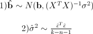
while the sigma squared with a lid is an unbiased estimate for the real sigma squared. Here b is the real vector of coefficients, and epsilon with a lid is the vector of residuals, if we take the least-squares estimates as coefficients. That is, assuming that errors are distributed normally, the vector of coefficients will also be distributed normally around the real value, and its dispersion can be unbiasedly estimated. This means that it is possible to test the hypothesis for the equality of the coefficients to zero, and therefore to check the significance of the predictors, that is, whether the value of Xi really influences the quality of the constructed model.
To test this hypothesis, we need the following statistics, which has a Student's distribution if the real value of the coefficient bi is 0:

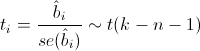
Where
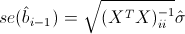- standard error of the coefficient estimate, and t (kn-1) - Student's distribution with kn-1 degrees of freedom.

Now everything is ready to continue parsing the output of the function summary.lm ().
So, next are the estimates of the coefficients obtained by the method of least squares, their standard errors, the values ​​of t-statistics and p-values for it. Usually, a p-value is compared with some sufficiently small pre-selected threshold, for example, 0.05 or 0.01. And if the value of p-statistics turns out to be less than the threshold, then the hypothesis is rejected; if more, nothing concrete, unfortunately, cannot be said. I recall that in this case, since the Student’s distribution is symmetrical with respect to 0, the p-value will be 1-F (| t |) + F (- | t |), where F is the Student’s distribution function with kn-1 degrees of freedom . Also, R kindly denotes asterisks significant coefficients for which the p-value is sufficiently small. That is, those coefficients that are with a very low probability are equal to 0. In the Signif line. codes just contain the decoding of asterisks: if there are three, then the p-value is from 0 to 0.001, if there are two, then it is from 0.001 to 0.01, and so on. If there are no icons, then the p-value is greater than 0.1.

In our example, it can be said with great confidence that the predictors of Elevation and Adjacent do affect the Species value with a high probability, but nothing definite can be said about the other predictors. Usually, in such cases, the predictors remove one by one and see how much other indicators of the model change, for example, BIC or Adjusted R-squared, which will be analyzed further.

The value of the Residual standart error corresponds simply to a sigma estimate with a lid, and the degrees of freedom are calculated as kn-1.

And now the most important statistics that you should look at first are: R-squared and Adjusted R-squared:

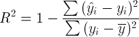
where Yi is the real Y values ​​in each observation, Yi with a lid are the values ​​predicted by the model, Y with the bar is the average for all real Yi values.


We begin with the statistics of the R-square or, as it is sometimes called, the coefficient of determination. It shows how the conditional dispersion of the model differs from the dispersion of real values ​​of Y. If this coefficient is close to 1, then the conditional dispersion of the model is quite small and it is very likely that the model describes the data quite well. If the R-squared coefficient is much less, for example, less than 0.5, then, with a large degree of confidence, the model does not reflect the real state of affairs.

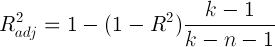
However, the R-square statistic has one serious drawback: with an increase in the number of predictors, this statistic can only increase. Therefore, it may seem that a model with a large number of predictors is better than a model with a smaller one, even if all new predictors do not affect the dependent variable in any way. Here you can recall the principle of Occam's razor . Following it, if possible, it is worth getting rid of the extra predictors in the model, as it becomes simpler and more understandable. For these purposes, a corrected R-square statistic was invented. It is a regular R-square, but with a penalty for a large number of predictors. The basic idea: if the new independent variables make a large contribution to the quality of the model, the value of these statistics increases, if not, then vice versa decreases.

For example, consider the same model as before, but now instead of five predictors, we’ll leave two:

 > lm2<-lm(Species~Elevation+Adjacent, data=gala) > summary(lm2) Call: lm(formula = Species ~ Elevation + Adjacent, data = gala) Residuals: Min 1Q Median 3Q Max -103.41 -34.33 -11.43 22.57 203.65 Coefficients: Estimate Std. Error t value Pr(>|t|) (Intercept) 1.43287 15.02469 0.095 0.924727 Elevation 0.27657 0.03176 8.707 2.53e-09 *** Adjacent -0.06889 0.01549 -4.447 0.000134 *** --- Signif. codes: 0 '***' 0.001 '**' 0.01 '*' 0.05 '.' 0.1 ' ' 1 Residual standard error: 60.86 on 27 degrees of freedom Multiple R-squared: 0.7376, Adjusted R-squared: 0.7181 F-statistic: 37.94 on 2 and 27 DF, p-value: 1.434e-08 

As you can see, the value of the R-squared statistics has decreased, but the value of the adjusted R-squared has even slightly increased.

Now we check the hypothesis that all coefficients are equal to zero under predictors. That is, the hypothesis about whether the value of Y generally depends on the values ​​of Xi linearly. To do this, you can use the following statistics, which, if the hypothesis that all coefficients are equal to zero, has the Fisher distribution cn and kn-1 degrees of freedom:

The value of F-statistics and p-value for it are in the last line of the output of the function summary.lm ().

Conclusion

In this article, standard methods for assessing the significance of coefficients and some criteria for assessing the quality of the constructed linear model were described. Unfortunately, I did not touch upon the question of considering the distribution of residuals and checking it for normality, since this would have doubled the article, although this is a rather important element of checking the adequacy of the model.
I really hope that I managed to slightly expand the standard idea of ​​linear regression, as an algorithm that just evaluates some kind of dependency, and to show how to evaluate its results.