Applying local binary patterns to solving face recognition tasks
Good day everyone!
The article has already briefly reviewed the LBP operator. I would like to dwell on this issue in more detail, and also consider the application of LBP to the solution of the problem of face recognition.
As a rule, the face recognition system is a software and hardware complex for automatic verification or identification of an individual from a digital image (photograph or frame of a video sequence). The task of face recognition is solved in the development of access control systems, border control systems, conducting operational search activities, etc.
')
In the process of face recognition, a number of difficulties arise associated with changes in lighting conditions, head rotation, age-related changes, and so on. The following main stages of the verification and identification process can be distinguished:
The main objectives of this work were the development and analysis of the facial recognition algorithm based on local binary patterns (LBT). We indicate the main stages of solving the task:
A local binary pattern is a specific type of feature used for classification in computer vision and is a simple operator. Local binary patterns were first proposed in 1996 for analyzing the texture of halftone images. Moreover, further studies have shown that LBPs are invariant to small changes in lighting conditions and small image rotations [1].
LBP is a description of the neighborhood of a pixel image in binary representation. The base LBR operator, applied to the image pixel, uses eight neighborhood pixels, taking the intensity value of the central pixel as a threshold (Figure 2.1). Pixels with an intensity value greater than or equal to the intensity value of the central pixel take values equal to "1", the rest take values equal to "0". Thus, the result of applying the base LBR operator to an image pixel is an eight-bit binary code that describes the neighborhood of this pixel [1].
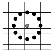
Using a circular neighborhood and bilinear interpolation of pixel intensity values allows you to build a local binary pattern with an arbitrary number of points P and radius R (Figure 2.2) [1-4].
Some binary codes carry more information than others. Thus, a local binary pattern is called uniform if it contains no more than three “0” and “1” series (for example, 00000000, 001110000 and 11100001). First, uniform LBPs determine only important local features of the image, such as the ends of lines, faces, angles, and spots (Figure 2.3). Second, they provide significant memory savings ( P ( P -1) +2 different patterns instead of 2 P ).
Applying the LBP operator to each pixel of the image, we can construct a histogram in which a separate column corresponds to each uniform LBP code. There is also another additional column that contains information about all non-uniform patterns.
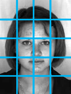
Face images can be considered as a set of various local features that are well described using local binary patterns. However, a histogram built for the entire image as a whole encodes only the presence of certain local features, but does not contain any information about their location in the image. To account for this kind of information, the image is divided into subregions, each of which calculates its LBP histogram (Figure 3.1). By concatenating these histograms, a common histogram can be obtained, taking into account both local and global features of the image [2, 3].
With this approach, for better extraction of features, it is possible to vary the parameters of the LBR operator and the number of image splits into subregions.
In the course of the work, three approaches were studied to calculate the measure of the difference between the histograms of two matched images and the construction of the corresponding decision rule.
Some subregions of the image may contain more important information than the others, and in accordance with this, each of them can be assigned its own weighting factor. Thus, for example, weights can be obtained using the Student’s criterion, which consists in testing the hypothesis of differences between two samples, according to training data representing two classes (“own” and “alien” in the case of solving the verification or identification problem).
As a measure of the difference between the two histograms, the Kullback-Leibler weighted distance was used in a symmetric form:
where ( i , j ) is the index of the subregion of the image, w ij is the weighting factor of the subregion, S 1 , S 2 are the LBR histograms of the first and second images, respectively , k is the column number of the LBR histogram, P is the number of neighborhood points in the LBS template.
In this case, the identification problem was solved using the classifier by the method of the nearest neighbor, and the verification problem was solved by the threshold classification.
This approach is to use the Mahalanobis distance:
where x , y are random vectors with the same distribution and the correlation matrix S.
The correlation matrix S can be obtained using a training sample of images. By determining the Kullback-Leibler distance (4.1) for each of the subdomains of images, we can obtain a vector of differences between two images. By calculating such vectors for each pair of images of the training set, we obtain two sets of image difference vectors corresponding to two classes — the class of “friends” and the class of “alien”. After that we can calculate the average values of the vectors representing each of the classes, as well as two correlation matrices.
In practice, for any two images, we can calculate their difference vector, and then determine the Mahalanobis distance d 1 and d 2 between this vector and average vectors of “own” and “alien” classes, respectively. Identification and verification can be made by comparing the two obtained distances or using the discriminating function f ( d 1 , d 2 ) = d 2 ⁄ ( d 1 + d 2 ) and a certain threshold value.
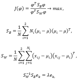
The following approach relies on the use of the Fisher linear discriminant (LDF):
where μ i is the average for the i -th class, μ is the general average, N i is the number of representatives in the i -th class, N is the total number of representatives in the training set, x ij is the j -th representative of the i -th class.
Let there be two sets of vectors corresponding to two classes. The eigenvector corresponding to the largest eigenvalue of the matrix S w -1 S b specifies a transformation to a space of dimension 1.
The task of identification and verification can be solved in a way similar to the previous one (by constructing image difference vectors using the Kullback-Leibler distance). In this case, instead of the Mahalanobis distance, the vector is mapped into one-dimensional space.
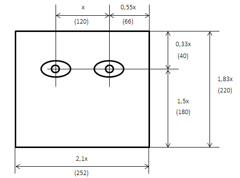
In order to reduce the noise level, median and Gaussian filters were used. In addition, the images underwent the normalization procedure, i.e. they were cropped, scaled and turned to the horizontal position of the line connecting the centers of the eyes (Figure 5.1).
The ColorFERET database was used for training and testing.
All algorithms were trained so as to ensure a false tolerance probability (FAR) value of 0.1%. The best results were obtained using the following parameters:
Table 6.1 shows the results of testing the developed algorithms.
This article briefly describes the algorithm for constructing a feature vector based on local binary patterns.
It is shown that the use of different decision rules for the same feature vectors can improve the quality of the face recognition system. As can be seen from table 6.1, the best probability characteristics are obtained using the Fisher linear discriminant.
In addition, it should be noted that the quality of the system depends significantly on the pre-processing of input images. In the course of the work, it was noted that the absence of a filtering step leads to a decrease in the likelihood of correct identification and verification.
PS I would like to separately note that in further work the probabilistic characteristics of the verification and identification algorithm were slightly improved. This was achieved by constructing feature vectors not only for the image of the face as a whole, but also for the areas of a pair of eyes, nose and mouth, as well as a significant increase in the size of the training set. Unfortunately, I can not present in more detail the materials of these studies, since the results obtained are a commercial secret.
PPS This article is based on my other publication and includes some corrections. A big request when using the materials of this article (especially in scientific papers) to refer to the original version:
Petruk V.I., Samorodov A.V., Spiridonov I.N. The use of local binary patterns to solve the problem of face recognition. Bulletin of the Moscow State Technical University. N.E. Bauman. Series: Instrument making. 2011. No. S. p. 58-63.
The article has already briefly reviewed the LBP operator. I would like to dwell on this issue in more detail, and also consider the application of LBP to the solution of the problem of face recognition.
1. Introduction
As a rule, the face recognition system is a software and hardware complex for automatic verification or identification of an individual from a digital image (photograph or frame of a video sequence). The task of face recognition is solved in the development of access control systems, border control systems, conducting operational search activities, etc.
')
In the process of face recognition, a number of difficulties arise associated with changes in lighting conditions, head rotation, age-related changes, and so on. The following main stages of the verification and identification process can be distinguished:
- image registration and normalization;
- feature selection;
- calculation of the proximity measure;
- building a decision rule.
The main objectives of this work were the development and analysis of the facial recognition algorithm based on local binary patterns (LBT). We indicate the main stages of solving the task:
- pre-processing (normalization) of the image;
- plotting the feature vector;
- the choice of a measure of proximity;
- building a decision rule;
- testing and comparing different approaches.
2. Local binary patterns
A local binary pattern is a specific type of feature used for classification in computer vision and is a simple operator. Local binary patterns were first proposed in 1996 for analyzing the texture of halftone images. Moreover, further studies have shown that LBPs are invariant to small changes in lighting conditions and small image rotations [1].
LBP is a description of the neighborhood of a pixel image in binary representation. The base LBR operator, applied to the image pixel, uses eight neighborhood pixels, taking the intensity value of the central pixel as a threshold (Figure 2.1). Pixels with an intensity value greater than or equal to the intensity value of the central pixel take values equal to "1", the rest take values equal to "0". Thus, the result of applying the base LBR operator to an image pixel is an eight-bit binary code that describes the neighborhood of this pixel [1].
 |
| Figure 2.1 - Basic LBP operator |
Using a circular neighborhood and bilinear interpolation of pixel intensity values allows you to build a local binary pattern with an arbitrary number of points P and radius R (Figure 2.2) [1-4].
 |
| Figure 2.2 - Extended LBP operator |
Some binary codes carry more information than others. Thus, a local binary pattern is called uniform if it contains no more than three “0” and “1” series (for example, 00000000, 001110000 and 11100001). First, uniform LBPs determine only important local features of the image, such as the ends of lines, faces, angles, and spots (Figure 2.3). Second, they provide significant memory savings ( P ( P -1) +2 different patterns instead of 2 P ).
 |
| Figure 2.3 - Examples of local features detected by RLBS |
3. Histogram LBSH
Applying the LBP operator to each pixel of the image, we can construct a histogram in which a separate column corresponds to each uniform LBP code. There is also another additional column that contains information about all non-uniform patterns.
Face images can be considered as a set of various local features that are well described using local binary patterns. However, a histogram built for the entire image as a whole encodes only the presence of certain local features, but does not contain any information about their location in the image. To account for this kind of information, the image is divided into subregions, each of which calculates its LBP histogram (Figure 3.1). By concatenating these histograms, a common histogram can be obtained, taking into account both local and global features of the image [2, 3].
 |
| Figure 3.1 - Splitting a face image into subdomains |
With this approach, for better extraction of features, it is possible to vary the parameters of the LBR operator and the number of image splits into subregions.
4. Building a decision rule
In the course of the work, three approaches were studied to calculate the measure of the difference between the histograms of two matched images and the construction of the corresponding decision rule.
4.1. Kullback-Leibler Weighted Distance
Some subregions of the image may contain more important information than the others, and in accordance with this, each of them can be assigned its own weighting factor. Thus, for example, weights can be obtained using the Student’s criterion, which consists in testing the hypothesis of differences between two samples, according to training data representing two classes (“own” and “alien” in the case of solving the verification or identification problem).
As a measure of the difference between the two histograms, the Kullback-Leibler weighted distance was used in a symmetric form:
 | (4.1) |
where ( i , j ) is the index of the subregion of the image, w ij is the weighting factor of the subregion, S 1 , S 2 are the LBR histograms of the first and second images, respectively , k is the column number of the LBR histogram, P is the number of neighborhood points in the LBS template.
In this case, the identification problem was solved using the classifier by the method of the nearest neighbor, and the verification problem was solved by the threshold classification.
4.2. Mahalanobis Distance
This approach is to use the Mahalanobis distance:
 | (4.2) |
where x , y are random vectors with the same distribution and the correlation matrix S.
The correlation matrix S can be obtained using a training sample of images. By determining the Kullback-Leibler distance (4.1) for each of the subdomains of images, we can obtain a vector of differences between two images. By calculating such vectors for each pair of images of the training set, we obtain two sets of image difference vectors corresponding to two classes — the class of “friends” and the class of “alien”. After that we can calculate the average values of the vectors representing each of the classes, as well as two correlation matrices.
In practice, for any two images, we can calculate their difference vector, and then determine the Mahalanobis distance d 1 and d 2 between this vector and average vectors of “own” and “alien” classes, respectively. Identification and verification can be made by comparing the two obtained distances or using the discriminating function f ( d 1 , d 2 ) = d 2 ⁄ ( d 1 + d 2 ) and a certain threshold value.
4.3. The use of linear discriminant Fisher
The following approach relies on the use of the Fisher linear discriminant (LDF):
 | (4.3) |
where μ i is the average for the i -th class, μ is the general average, N i is the number of representatives in the i -th class, N is the total number of representatives in the training set, x ij is the j -th representative of the i -th class.
Let there be two sets of vectors corresponding to two classes. The eigenvector corresponding to the largest eigenvalue of the matrix S w -1 S b specifies a transformation to a space of dimension 1.
The task of identification and verification can be solved in a way similar to the previous one (by constructing image difference vectors using the Kullback-Leibler distance). In this case, instead of the Mahalanobis distance, the vector is mapped into one-dimensional space.
5. Image preprocessing
In order to reduce the noise level, median and Gaussian filters were used. In addition, the images underwent the normalization procedure, i.e. they were cropped, scaled and turned to the horizontal position of the line connecting the centers of the eyes (Figure 5.1).
 |
| Figure 5.1 - Image Normalization Parameters |
6. Description and results of the experiment
The ColorFERET database was used for training and testing.
- training sample: 100 people, 5 photos for each;
- test sample: 329 people, 2 photos for each.
All algorithms were trained so as to ensure a false tolerance probability (FAR) value of 0.1%. The best results were obtained using the following parameters:
- LBSH operator parameters: P = 8, R = 2;
- Number of image splits: 6 × 6 (along the x and y axes, respectively).
Table 6.1 shows the results of testing the developed algorithms.
| Measure of difference | Closed set identification | Verification |
| Kullback-Leibler Weighted Distance | 89.5% | 84.2% |
| Mahalanobis Distance | 89.8% | 80.8% |
| Conversion to 1-dimensional space using LDF | 92.0% | 86.0% |
7. Conclusion
This article briefly describes the algorithm for constructing a feature vector based on local binary patterns.
It is shown that the use of different decision rules for the same feature vectors can improve the quality of the face recognition system. As can be seen from table 6.1, the best probability characteristics are obtained using the Fisher linear discriminant.
In addition, it should be noted that the quality of the system depends significantly on the pre-processing of input images. In the course of the work, it was noted that the absence of a filtering step leads to a decrease in the likelihood of correct identification and verification.
8. List of sources used
- T. Maenpaa. Texture Extensions and Applications. Oulu University Press , 2003.
- D. Maturana, D. Mery, A. Soto. Face Recognition with Spatial Pyramid Histograms and Naive Bayes Nearest Neighbor classification. In Proc. of the XXVIII International Conference of the Chilean Computer Science Society, IEEE CS Society , 2009.
- C. Shan, S. Gong, PW McOwan. A comprehensive study of facial expression patterns. Image and Vision Computing , (27), 2009.
- T. Ahonen, A. Hadid, M. Pietikainen. Face Recognition with Local Binary Patterns. Lecture Notes in Computer Science , 2004.
PS I would like to separately note that in further work the probabilistic characteristics of the verification and identification algorithm were slightly improved. This was achieved by constructing feature vectors not only for the image of the face as a whole, but also for the areas of a pair of eyes, nose and mouth, as well as a significant increase in the size of the training set. Unfortunately, I can not present in more detail the materials of these studies, since the results obtained are a commercial secret.
PPS This article is based on my other publication and includes some corrections. A big request when using the materials of this article (especially in scientific papers) to refer to the original version:
Petruk V.I., Samorodov A.V., Spiridonov I.N. The use of local binary patterns to solve the problem of face recognition. Bulletin of the Moscow State Technical University. N.E. Bauman. Series: Instrument making. 2011. No. S. p. 58-63.
Source: https://habr.com/ru/post/193658/
All Articles