Accounting of statistical information about traffic jams when searching for driving by car
Not so long ago, an article about routing algorithms in 2GIS products was published on Habré. I will continue the story of a colleague, explaining on what principles in the PC version we are looking for the best time route for the car. Here I would like to remind you that the PC version of 2GIS works without an internet connection.
Let's start with the fact that the required route from point A to point B may have different requirements:
- route length (shortest);
- travel time on the route (taking into account traffic jams);
- intermediate points (preferences on the route), etc.
The current routing algorithm supports two types of routes - optimal in length (shortest in distance) and optimal in time (shortest in travel time). If everything is clear with the criterion for assessing the shortest route by distance, then it is often very difficult to correctly estimate the travel time in a modern city overloaded with transport. Travel time on the same route may vary significantly depending on the time of day, day of the week, repairs being carried out, weather conditions, accidents, etc. In other words, when plotting a time-optimal route, it is necessary to be able to accurately estimate the current situation on the road accurately or to be able to approximate it fairly close.
')
In this connection, a rather natural idea arose: when searching for a route that is optimal in time, use the statistics accumulated by the Traffic Service (Novosibirsk). These statistics reflect road congestion depending on the time of day, day of the week and season. In this case, in the case of an online version of the location search service, it becomes possible to use the most recent data, which can additionally take into account ongoing repairs, weather conditions and accidents. Further in this article we will discuss the use of such information when searching for travel in offline products.
It all starts with collecting statistics on traffic jams. It gathers along all the edges of the city’s road graph and accumulates for every 15 minutes of each day of the week. The preparation of statistics consists of two main stages:

For a fixed day of the week, for all edges of the road graph, which participate in the calculation of traffic jams, and for each 15-minute time interval:
The current “Usually” statistics for Novosibirsk can be viewed on the Traffic jams service - the main purpose of these statistics. The vector of statistical velocities on the edge for the week, divided into 15-minute intervals, will be called the time profile of this edge. The time profile characterizes the dynamics of the speed change on the edge during the week (it is convenient to depict as a graph) and consists of 672 elements. In this case, each of the elements is an integer one-byte number and is equal to the speed on this edge in the corresponding 15-minute time interval.
Direct use of statistics "Usually" to estimate the time of travel along the route is difficult in practice. The road graph of a large city consists of tens and hundreds of thousands of ribs. To keep a separate time profile for each edge is very expensive, or even impossible. To circumvent this problem, it was decided to merge all available temporary profiles into a small number of classes. Each such class is an averaged smoothed time profile describing the dynamics of the speed of a traffic flow on a certain group of edges of a road graph. Further, all edges of the graph are distributed between the selected classes (classified), and routing procedures instead of temporary edge profiles can work with edge class time profiles.
To build classes of temporal profiles of the edges, factor analysis was used . The choice of this method is determined by the capabilities of the factor analysis to identify hidden (but supposed) patterns in the process being studied, to identify statistical relationships and compress information by describing the original process using common factors, the number of which is (substantially) less than the number of features originally taken. In our case, the initial signs are the edge profiles, and the common factors are the classes of the time profiles.
The use of factor analysis can be divided into three main stages.
The covariance matrix of time profiles has the following form, where E is the expectation value:

To circumvent the obstacles listed above, it was decided to build covariance matrices for fragments of the road graph. Experimentally, we determined that, for our data, the use of dimension matrices, preferably not more than 1,000, allows us to obtain qualitative results for each sample in a reasonable time. Moreover, the road graph is divided into a relatively small number of such fragments — on the order of several dozen. The division of the road graph into fragments (subsets of edges) is performed dynamically with each start of the classification procedure for time profiles.
The next classification step is to rank all the constructed factors by significance. To do this, all the time profiles of the edges that make up the fragment of the road graph being processed are distributed among the factors - the profile refers to the factor from which it has the minimum deviation. Deviation is calculated by the method of least squares . As a result, each factor gets a rank — the number of time profiles associated with it. The factor with the lowest rank is discarded, and the time profiles associated with it are distributed among the remaining factors.
The described procedure continues until the number of the most significant facts necessary for us remains, between which all the temporal profiles of the edges from this fragment of the graph are already distributed. Such remaining factors become classes, and the edges associated with them receive their classes — time profiles of factors.
An example of the constructed classes for a fragment of the road graph of Novosibirsk is shown in the figure below. On the X axis, the time in minutes from the beginning of the week changes, on the Y axis - the speed in km / h. The class graph shows the speed change on the edges of a given class over time over the week. Fluctuations of the graph reflect the dependence of the speed of the traffic flow on the time of day on the edges of this class. It can be seen from the figure that the constructed classes differ markedly in their characteristics — each class has its own speed range.

In total, about 100 such classes are obtained for Novosibirsk. The distribution of all the temporal edge profiles for these classes makes it possible to store a rather compact set of classes instead of the original profiles, occupying only ~ 65–70 Kb on the disk. We call such a set of classes a velocity matrix.
The preparation of the velocity matrix is part of the road graph preparation procedure, and the matrix itself is part of the binary file that the road graph is packed into. The algorithm for finding the route on the graph was described in detail in the previous article . The velocity from the velocity matrix is used in estimating the accumulated travel time on the viewed edges. Thus, this information becomes key when searching for routes that are optimal in terms of travel time, taking into account traffic jams.
Consider a typical picture of traffic jams in Novosibirsk on Monday at 18:00 local time (“Usually” statistics):

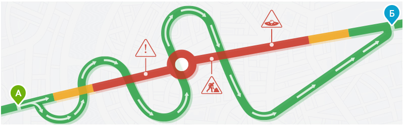
Compare two routes from point A to point B - the shortest in distance and optimal in travel time. The shortest route: length - 7,330 meters, travel time taking into account information about traffic jams - 1,347 seconds:

Optimal travel time: length - 8,033 meters, travel time taking into account traffic information - 1,295 seconds:

Thus, the described technique makes it possible to “pack” statistical information about velocities at tens of thousands of edges of a road graph into a relatively small object of ~ 65–70 Kb. This makes it possible to use it in offline products. The considered example shows that the optimal route in time is consistent with the traffic jams observed at the indicated time point (we drive around the slower sections through which the shortest route passes).
Let's start with the fact that the required route from point A to point B may have different requirements:
- route length (shortest);
- travel time on the route (taking into account traffic jams);
- intermediate points (preferences on the route), etc.
The current routing algorithm supports two types of routes - optimal in length (shortest in distance) and optimal in time (shortest in travel time). If everything is clear with the criterion for assessing the shortest route by distance, then it is often very difficult to correctly estimate the travel time in a modern city overloaded with transport. Travel time on the same route may vary significantly depending on the time of day, day of the week, repairs being carried out, weather conditions, accidents, etc. In other words, when plotting a time-optimal route, it is necessary to be able to accurately estimate the current situation on the road accurately or to be able to approximate it fairly close.
')
In this connection, a rather natural idea arose: when searching for a route that is optimal in time, use the statistics accumulated by the Traffic Service (Novosibirsk). These statistics reflect road congestion depending on the time of day, day of the week and season. In this case, in the case of an online version of the location search service, it becomes possible to use the most recent data, which can additionally take into account ongoing repairs, weather conditions and accidents. Further in this article we will discuss the use of such information when searching for travel in offline products.
Statistics collection
It all starts with collecting statistics on traffic jams. It gathers along all the edges of the city’s road graph and accumulates for every 15 minutes of each day of the week. The preparation of statistics consists of two main stages:
- The accumulation of data by day of the week . All points from the devices collected per day are grouped by the edges of the graph and 15-minute time intervals. Next, for each edge for each time interval, speed averaging is performed. We will call such statistics primary. It is stored in the database for the last 4 weeks. Data older than 4 weeks are deleted.
- Aggregation of accumulated data . After adding the data for the new day, we recalculate the so-called. "Usually" statistics for the corresponding day of the week.
For a fixed day of the week, for all edges of the road graph, which participate in the calculation of traffic jams, and for each 15-minute time interval:
- We retrieve the primary statistics of this day for the last 4 weeks:
- average speed on the edge,
- the total number of points from the devices on this edge,
- the total number of devices from which the points came. - We fold with different weights of speed for all 4 weeks. Each week has its own weight coefficient, which depends on the relevance of the data (those that are the most recent for the last week, have the maximum weight) and their reliability (the number of devices and the number of points from them on a specific edge).
The current “Usually” statistics for Novosibirsk can be viewed on the Traffic jams service - the main purpose of these statistics. The vector of statistical velocities on the edge for the week, divided into 15-minute intervals, will be called the time profile of this edge. The time profile characterizes the dynamics of the speed change on the edge during the week (it is convenient to depict as a graph) and consists of 672 elements. In this case, each of the elements is an integer one-byte number and is equal to the speed on this edge in the corresponding 15-minute time interval.
Data analysis method
Direct use of statistics "Usually" to estimate the time of travel along the route is difficult in practice. The road graph of a large city consists of tens and hundreds of thousands of ribs. To keep a separate time profile for each edge is very expensive, or even impossible. To circumvent this problem, it was decided to merge all available temporary profiles into a small number of classes. Each such class is an averaged smoothed time profile describing the dynamics of the speed of a traffic flow on a certain group of edges of a road graph. Further, all edges of the graph are distributed between the selected classes (classified), and routing procedures instead of temporary edge profiles can work with edge class time profiles.
To build classes of temporal profiles of the edges, factor analysis was used . The choice of this method is determined by the capabilities of the factor analysis to identify hidden (but supposed) patterns in the process being studied, to identify statistical relationships and compress information by describing the original process using common factors, the number of which is (substantially) less than the number of features originally taken. In our case, the initial signs are the edge profiles, and the common factors are the classes of the time profiles.
Classification of temporal edge profiles
The use of factor analysis can be divided into three main stages.
1. Covariance matrix
The analysis begins with the construction of a covariance matrix of edge time profiles, which is necessary to isolate factors. Denote the time profile of the edge by the vector v = (v [1], ..., v [m]), where v [i] is the speed of the traffic flow on the edge at time i = 1, ..., m. Now the time period of the “Usually” statistics is 1 week with 15-minute sampling, which gives m = 7 × 24 × 60/15 = 672.The covariance matrix of time profiles has the following form, where E is the expectation value:
2. Decomposition of the original problem
To build the desired classes of time profiles, it is required to find the eigenvectors and eigenvalues of the covariance matrix - in fact, everything comes down to solving systems of linear equations. In practice, the full covariance matrix for such a city, for example, as Novosibirsk will occupy about 6 Gb. On the other hand, all modern algorithms for finding eigenvalues and matrix vectors have a cubic complexity of the dimension of the matrix. In addition, as the matrix dimension increases, the computation error increases.To circumvent the obstacles listed above, it was decided to build covariance matrices for fragments of the road graph. Experimentally, we determined that, for our data, the use of dimension matrices, preferably not more than 1,000, allows us to obtain qualitative results for each sample in a reasonable time. Moreover, the road graph is divided into a relatively small number of such fragments — on the order of several dozen. The division of the road graph into fragments (subsets of edges) is performed dynamically with each start of the classification procedure for time profiles.
3. Building classes of temporary profiles
For each subset obtained as a result of the decomposition of the original problem, a covariance matrix is constructed, for which we need to find the eigenvectors and eigenvalues. To do this, use the library of linear algebra Eigen , which showed the best performance and quality of the account on our problems. We will not go deep into the used computational procedures and their mathematical justification (those who wish can refer to the special literature). Just note that eigenvalues and vectors are necessary to determine the so-called. factors (factor analysis terminology) is the result of combining time profiles that strongly correlate with each other. In our problem, by construction, the factors themselves are time profiles, obtained as a linear combination of correlated time profiles of the original edges.The next classification step is to rank all the constructed factors by significance. To do this, all the time profiles of the edges that make up the fragment of the road graph being processed are distributed among the factors - the profile refers to the factor from which it has the minimum deviation. Deviation is calculated by the method of least squares . As a result, each factor gets a rank — the number of time profiles associated with it. The factor with the lowest rank is discarded, and the time profiles associated with it are distributed among the remaining factors.
The described procedure continues until the number of the most significant facts necessary for us remains, between which all the temporal profiles of the edges from this fragment of the graph are already distributed. Such remaining factors become classes, and the edges associated with them receive their classes — time profiles of factors.
An example of the constructed classes for a fragment of the road graph of Novosibirsk is shown in the figure below. On the X axis, the time in minutes from the beginning of the week changes, on the Y axis - the speed in km / h. The class graph shows the speed change on the edges of a given class over time over the week. Fluctuations of the graph reflect the dependence of the speed of the traffic flow on the time of day on the edges of this class. It can be seen from the figure that the constructed classes differ markedly in their characteristics — each class has its own speed range.
In total, about 100 such classes are obtained for Novosibirsk. The distribution of all the temporal edge profiles for these classes makes it possible to store a rather compact set of classes instead of the original profiles, occupying only ~ 65–70 Kb on the disk. We call such a set of classes a velocity matrix.
Speed Matrix Routing Algorithm
The preparation of the velocity matrix is part of the road graph preparation procedure, and the matrix itself is part of the binary file that the road graph is packed into. The algorithm for finding the route on the graph was described in detail in the previous article . The velocity from the velocity matrix is used in estimating the accumulated travel time on the viewed edges. Thus, this information becomes key when searching for routes that are optimal in terms of travel time, taking into account traffic jams.
Consider a typical picture of traffic jams in Novosibirsk on Monday at 18:00 local time (“Usually” statistics):
Compare two routes from point A to point B - the shortest in distance and optimal in travel time. The shortest route: length - 7,330 meters, travel time taking into account information about traffic jams - 1,347 seconds:
Optimal travel time: length - 8,033 meters, travel time taking into account traffic information - 1,295 seconds:
Thus, the described technique makes it possible to “pack” statistical information about velocities at tens of thousands of edges of a road graph into a relatively small object of ~ 65–70 Kb. This makes it possible to use it in offline products. The considered example shows that the optimal route in time is consistent with the traffic jams observed at the indicated time point (we drive around the slower sections through which the shortest route passes).
Source: https://habr.com/ru/post/193116/
All Articles