Introduction

One of the tasks of teaching without a teacher is the problem of finding the topological structure that most accurately reflects the topology of the distribution of input data. There are several approaches to solving this problem. For example, the Kohonen Self-Organizing Maps algorithm is a method of projecting multidimensional space into a space with a lower dimension (usually two-dimensional) with a predetermined structure. In connection with a decrease in the dimension of the original problem, and a predetermined structure of the network, projection defects arise, the analysis of which is a difficult task. As one of the alternatives to this approach, the combination of Hebb’s competitive learning and neural gas is more effective in building a topological structure. But the practical application of this approach is hampered by a number of problems: a priori knowledge is needed of the required network size and the complexity of applying adaptation methods to the training speed of this network, excessive adaptation leads to a decrease in efficiency when teaching new data, and too slow adaptation speed causes high sensitivity to noisy data.

For online learning or long-term learning tasks, the methods listed above are not suitable. The fundamental problem for such tasks is how the system can adapt to new information without damaging or destroying the already known one.

This article discusses the SOINN algorithm, which partially solves the problems voiced above.

')

Review of the algorithm under consideration

In the task of teaching without a teacher, we need to divide the incoming data into classes, without prior knowledge of their number. It is also necessary to determine the topology of the source data.

So, the algorithm must meet the following requirements:

• Online training, or lifetime
• Division into classes without prior knowledge of input data
• Sharing data with a fuzzy boundary and identifying the main cluster structure

SOINN is a two-layer neural network. The first layer is used to determine the topological structure of the clusters, and the second to determine the number of clusters and to identify prototype nodes for them. First, the first layer of the network is trained, and then, using the data obtained by training the first layer, the second layer of the network is learned.

For the task of classification without a teacher, it is necessary to determine whether the input image belongs to one of the previously obtained clusters or represents a new one. Suppose that two images belong to the same cluster, if the distance (by a predetermined metric) between them is less than the threshold distance T. If T is too large, then all input images will be assigned to the same cluster. If T is too small, then each image will be isolated as a separate cluster. To obtain a reasonable division into clusters, T must be greater than the intraclass distance and less than the interclass distance.

For each of the layers of the SOINN network, we must calculate the threshold T. The first layer does not have a priori knowledge of the structure of the source data, so T is chosen adaptively, based on the knowledge of the structure of the already constructed network and the current input image. When learning the second layer, we can calculate the intraclass and interclass distance and choose the constant value of the threshold T.

To represent the topological structure, in online or lifetime learning tasks, network growth is an important element for reducing errors and adapting to changing conditions, keeping old data. But at the same time, an uncontrolled increase in the number of nodes leads to network overload and "retrain" it as a whole. Therefore, it is necessary to decide when and how to add new nodes to the network, and when to prevent the addition of new nodes.

To add nodes, SOINN uses a scheme in which the insertion occurs in a region with the maximum error. And to assess the utility of the insert, the “error radius” is used, which is the estimate of the utility of the insert. This assessment ensures that the insertion reduces the error and controls the growth of the nodes, and eventually stabilizes their number.

To compose connections between neurons, the Hebba competitive rule proposed by Martinez in the topology distribution network (TRN) is used. Hebba's competitive rule can be described as follows: for each input signal, the two closest nodes are combined. It is proved that each graph optimally represents the topology of the input data. In online or lifetime learning tasks, nodes change their location slowly, but constantly. Thus, nodes that are adjacent at an early stage may not be close at a later stage. Thus, it becomes necessary to remove connections that have not been updated recently.

In the general case, overlapping of existing clusters also occurs. To determine the number of clusters accurately, it is assumed that the input data are shared: the probability density in the central part of each cluster is higher than the density in the part between the clusters, and the cluster overlap has a low probability density. Separation of clusters occurs by removing nodes from regions with a low probability density. The SOINN algorithm proposes the following strategy for removing nodes from regions with a low probability density: if the number of signals generated so far is an integral multiple of a given parameter, then remove those nodes that have only one topological neighbor or have no neighbors at all and if the local accumulated the signal level is small, then we consider such nodes lying in the region of low probability density and remove them.

Algorithm Description

Now, based on the above, we can give a formal description of the learning algorithm for the SOINN network. This algorithm is used for training and the first and second layers of the network. The only difference is that the input data for learning the second layer is generated by the first layer and when learning the second layer, we have knowledge about the topological structure of the first layer to calculate the constant similarity threshold.

Used notation

• A is the set used to store nodes.
• NA - the number of nodes in the set A
• C - many connections between nodes
• NC is the number of edges in C
• Wi - n-dimensional weight vector for node i
• Ei - local error accumulator for node i
• Mi - local signal accumulator for node i
• Ri is the error radius for node i. Ri = Ei / Mi
• Ci - cluster label for node i
• Q is the number of clusters
• Ti is the similarity threshold for node i
• Ni - set of topological neighbors for node i
• age (i, j) is the age of communication between nodes i and j

Algorithm

1. Initialize the set of nodes A with two nodes, c1 and c2:
   A = {c1, c2}
   Initialize a set of edges C with an empty set:
   C = {}.
2. Input the new signal x from R ^ n.
3. Find in the set A the nodes of the winner s1 and the second winner, as nodes with the closest and following vectors of weights (by some given metric). If the distance between x, s1 and s2 is greater than the similarity thresholds Ts1 or Ts2, then create a new node and go to step 2.
4. If the edge between s1 and s2 does not exist, then create it. Set the age of the edge between them to 0.
5. Increase the age of all arcs leaving s1 by 1.
6. Add the distance between the input signal and the winner to the local total error Es1.
7. Increase the local number of s1 node signals:
   Ms1 = Ms1 +1
8. Adapt the scales of the winner and his direct topological neighbors:
   Ws1 = Ws1 + e1 (t) (x - Ws1)
   Wsi = Wsi + e2 (t) (x - Wsi)
   Where e1 (t) and e2 (t) are the learning coefficients of the winner and his neighbors.
9. Remove edges with age, above a given threshold.
10. If the number of input signals generated so far is a multiple of the lambda parameter, insert a new node and remove nodes in low probability density areas according to the following rules:
    
    1. Find the node q with the maximum error.
    2. Find among the neighbors q the node f with the maximum error.
    3. Add the node r so that its weight vector is the arithmetic average of the weights q and f.
    4. Calculate the accumulated error Er, the total number of signals Mr, and the inherited error radius:
       Er = alpha1 * (Eq + Ef)
       Mr = alpha2 * (Mq + Mf)
       Rr = alpha3 * (Rq + Rf)
    5. Reduce the total error of the nodes q and r:
       Eq = beta * Eq
       Ef = beta * Ef
    6. Reduce the accumulated number of signals:
       Mq = gamma * Mq
       Mf = gamma * Mf
    7. Determine whether the new node was successfully inserted. If the insertion cannot reduce the average error of this area, then the insertion failed. The added vertex is deleted, and all parameters are returned to their original states. Otherwise we update the error radius of all nodes involved in the insertion:
       Rq = Eq / Mq
       Rf = Ef / Mf
       Rr = Er / Mr.
    8. If the insertion was successful, create relations q <-> r and r <-> f and remove the connection q <-> f.
    9. Among all the nodes in A, find those that have only one neighbor, then compare the accumulated number of input signals with the average of all the nodes. If the node contains only one neighbor and the signal counter does not exceed the adaptive threshold, remove it from the node set. For example, if Li = 1 and Mi <c * sum_ {j = 1 ... Na} Mj / Na (where 0 <c <1), then delete the vertex i.
    10. Remove all isolated nodes.
11. After a long time LT, each class of input data will correspond to a connected component in the constructed graph. Update class labels.
12. Go to step 2 and continue learning.

The algorithm for calculating the threshold value T

For the first layer, the similarity threshold T is calculated adaptively using the following algorithm:

1. Initialize the similarity threshold for new nodes to be + oo.
2. When the node is the first or second winner, update the similarity threshold value:
   
   1. If the node has direct topological neighbors (Li> 0), update the value of Ti as the maximum distance between the node and its neighbors:
      Ti = max || Wi - Wj ||
   2. If the node has no neighbors, Ti is set as the minimum distance between the node and the other nodes in set A:
      Ti = min || Wi - Wc ||

For the second layer, the similarity threshold is constant and is calculated as follows:

1. Calculate the intraclass distance:
   dw = 1 / Nc * sum _ {(i, j) in C} || Wi - Wj ||
2. Calculate the interclass distance. The distance between classes Ci and Cj is calculated as follows:
   db (Ci, Cj) = max_ {i in Ci, j in Cj} || Wi - Wj ||
3. As the similarity threshold Tc, take the minimum interclass distance that exceeds the intraclass distance.

Schematic diagram of the algorithm

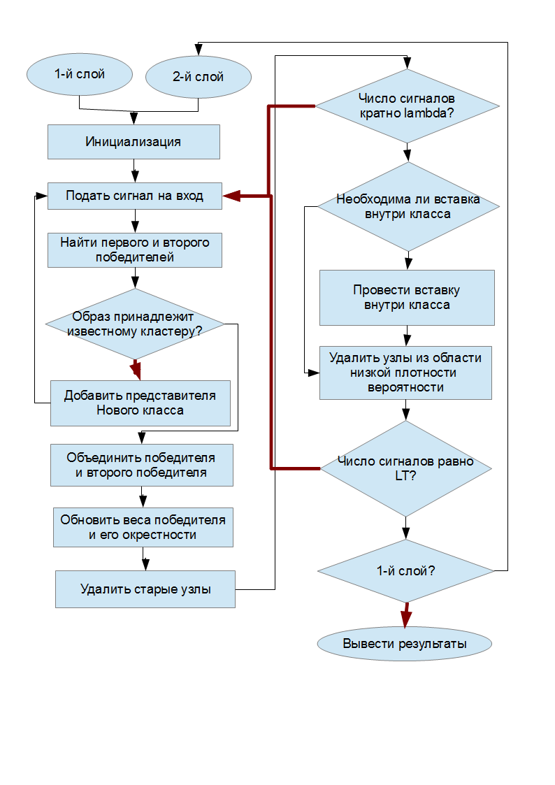
In the “conditional” diamond, the black arrows correspond to the fulfillment of the condition, and the red ones to non-fulfillment.

Experiments

To conduct experiments with the considered algorithm, it was implemented in C ++ using the Boost Graph Library. The code can be downloaded here .

For the experiments, the following algorithm parameters were chosen:

1. lambda = 100
2. age_max = 100
3. c = 1.0
4. alpha1 = 0.16
5. alpha2 = 0.25
6. alpha3 = 0.25
7. beta = 0.67
8. gamma = 0.75

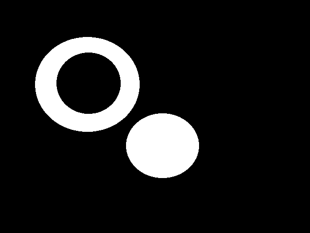
The following image was used as test data, representing two classes (ring and circle)

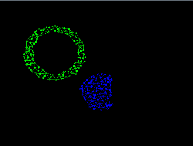
After submitting to the input of the network SOINN 20000 randomly taken points from these classes, the first layer of the network was formed, as follows

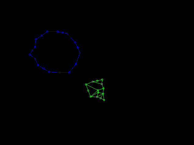
Based on the data obtained on the first layer, a second layer of the following type was formed.

findings

In this article, we looked at one of the unsupervised learning algorithms based on data topology. From the results obtained experimentally, we can conclude that the application of this method is fair.
But still worth noting the shortcomings of the algorithm SOINN:

1. Since the layers of the network are trained sequentially one after the other, it is difficult to determine the moment when it is necessary to stop learning the first layer and start learning the second layer.
2. When changing the first layer of the network, you must completely retrain the second layer. In this regard, the problem of online learning has not been solved.
3. The network has many parameters that must be selected manually.

References

“An incremental network for on-line unsupervised classi fi cation and topology learning” Sgen Furao, Osamu Hasegawa, 2005