Basic principles of digital wireless communication. Likbez
Hello. In this article, I would like to tell you a little about the basic techniques and ideas of modern digital wireless communications - using the example of the IEEE 802.11 standard. Nowadays, very often people live at rather high levels of abstraction, poorly imagining exactly how things around us work. Well, I will try to bring the light of enlightenment to the masses. The article will use the things and terminology explained in this article . So people who are far from radio engineering are advised to first read it.
DANGER: there is a matane in the article - especially impressionable not to press this button:
Digital signals and spectra
Analog signals
Before the development of computers, analog signals were usually transmitted via radio waves — that is, signals whose set of values is continuous .
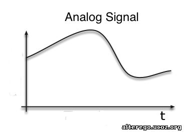
For example - sound - the dependence of pressure on time. The signal (voltage) received from the receiver goes to the audio amplifier and causes the speaker to oscillate.
')
Or a video signal for a kinescope. The signal level determines the value of the power running around the screen beam, which at the right moments of time illuminates the phosphor, forming an image on the screen
The main disadvantage of this method of transmitting information - low noise immunity - the transmitting medium always brings some random component to our signal - changing the shape of the video signal changes the colors of individual pixels (we all remember the noise of the radio receiver and the ripples on the TV screen).
Digital signals
Digital signals — that is, signals that have a discrete set of values — are much better than analog signals in this parameter, since we are not interested in the signal value itself, but in the range in which this value is located and we are not afraid of it (for example, in the 0V - 1.6V voltage range we we believe that this is a log 0, and in the range 3.3V - 5V log 1). The price paid for this is an increase in the required speed of information transmission and processing.
The first thing people have learned to do is to naturally transmit such signals by wire, simply by switching the state of the data line and synchronization from one to zero.
At this small educational program is completed - then we will discuss how the digital signal is transmitted using radio waves. How does wifi work.
Single pulse spectrum
In radio communications, we are often interested in the spectrum of a signal — a digital signal — a sequence of rectangular pulses — to begin with, consider the spectrum of a single rectangular pulse.
Recall what the spectrum is (the coefficient before the integral is omitted):
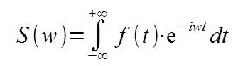
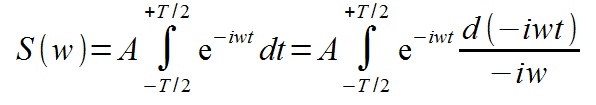
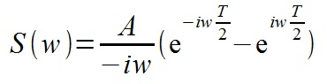
Spectrum of a rectangular pulse of duration T and amplitude A :
Conclusion
We take out the constant for the integral and make the replacement of the differential
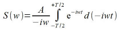
We consider a definite integral
Next, we make a replacement for the sine according to the Euler Formula
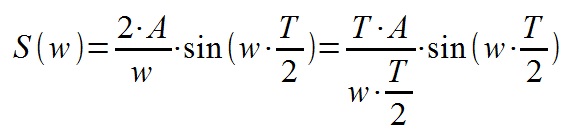
We take out the constant for the integral and make the replacement of the differential
We consider a definite integral
Next, we make a replacement for the sine according to the Euler Formula
Taak - what about the negative amplitude? Recall that in real numbers the spectrum decomposes into a sum of sines and cosines with zero phases -

in this form it is actually more convenient to present in a computer, but for analysis such a form is completely inconvenient - when the signal changes in the time domain - the spectra will change in a completely incomprehensible way for humans, therefore two spectra of the sinus components and cosine components are transformed into polar coordinates, folding pairs sine and cosine with zero phase to sine with non-zero phase, getting amplitude spectrum and phase, and now remember that multiplying a signal by -1 is equivalent to a phase jump of 180 degrees, therefore The main part will be reflected relative to the horizontal axis, and at the points of inflection the phase will experience a jump of 180 degrees.
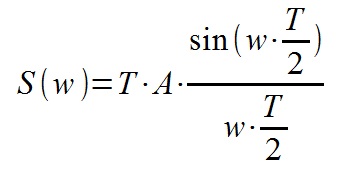
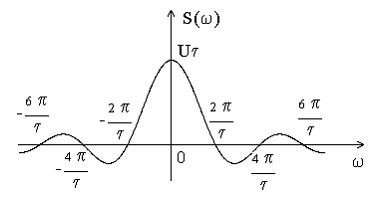
We also see that the spectrum of a single pulse is a sinc function , which is quite common in digital signal processing and radio engineering.
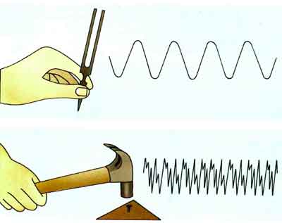
Almost all pulse energy is contained in the central peak of the spectrum — its width is inversely proportional to the pulse duration. And the height is directly proportional - that is, the longer the pulse is, the narrower and higher its spectrum, and the shorter the lower and wider.
The pulse sequence spectrum with a good degree of accuracy can be considered a set of harmonics in the spectral band, the width of which is inversely proportional to the pulse duration T.
So - the conclusion - by reducing the length of the pulses of our digital signal, we can smear the signal over a wide band of the spectrum - while its height decreases proportionally - if we increase the band by N times - the spectrum height will decrease to the same level as noise. Broadband transmission has quite a few advantages - one of them - resistance to narrowband interference - since the information is spread over the spectrum - narrowband interference spoils only a small part of this information.
If you stupidly reduce the length of the pulses of our information signal - the spectrum, of course, will broaden, but the receiver does not know what information we are transmitting to it and will not be able to extract it from the noise. Therefore, a method is needed - to convert a narrowband signal to a broadband noise-like signal for transmission over the radio channel, and after receiving it to convert back to narrowband - you need to add redundant information to the signal, that is, information known to both the receiver and the transmitter, with which the receiver can distinguish the signal from noise . We encode every bit of information known and the receiver and transmitter sequence.
Autocorrelation function. Barker codes
Our task is to find a known short sequence in the long sequence of input data.
Autocorrelation is a statistical relationship between random variables from a single series, but taken with a shift.
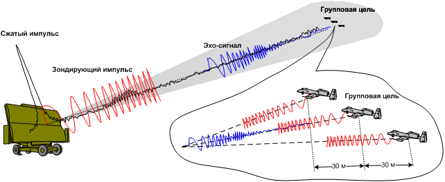
Of particular importance this parameter has in the location - we have generated some signal and spotted the time - the signal propagation speed is known to us, so knowing the time it took the signal to run to the obstacle and back - we can calculate the distance for the obstacle. But bad luck - there are no ideal conditions in life - as a rule, there are a lot of noises around and, together with the reflected signal, any garbage enters the receiver input. And first of all, we should not confuse our signal with anything else, and secondly, we need to accurately determine the point in time when he came back.
Mathematically, autocorrelation is defined as:
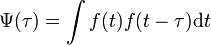
That is, we impose a function on ourselves, but with a shift, we multiply and calculate the integral, mark the point, then shift it again, again calculate the integral, and so on for all possible shifts. If we apply a function not to ourselves, but to some other one, then this is simply called a correlation .
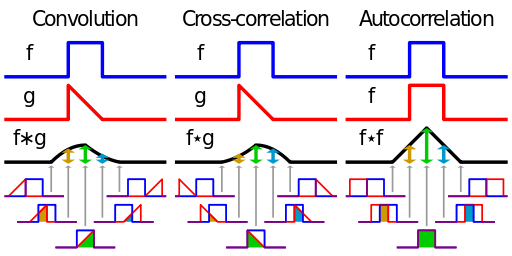
The image below shows convolution , correlation, and autocorrelation operations.
The difference between convolution and correlation — in the direction — convolution of the functions f (x) and g (x) is the same correlation, only functions f (x) and g (-x), autocorrelation is the correlation of the function with itself
That is, at the moment of time when the input signal is most similar to the function we need - the correlation function will have a peak. The width of this peak, if you do not take into account the noise - will be equal to twice the length of the probe pulse and will be symmetrical with respect to the central peak - even if the signal under study is not symmetrical. By the way - there may be several peaks - the central peak and the so-called side lobes - depends on the function. The correlation method is the most optimal method for determining a signal of known shape against a background of white noise — in other words, the method has the best signal-to-noise ratio. The probing pulse must meet the following requirements - have a narrow central peak as possible and at the same time have a minimum level of side lobes, that is, the function is similar to itself only in a very short time interval - move slightly and it becomes completely different. In the location of these requirements meets the chirp signal .
Having a minimal level of side lobes, the autocorrelation function of the chirp signal has the following form:
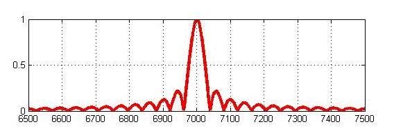
An analogue of the chirp signal in discrete systems is the Barker sequence
For example - the known sequence of 11 bits long: 11100010010.
Find the autocorrelation function of this sequence, cyclically shifting it and counting the sum of pairwise products, while replacing 0 with -1
11100010010
11100010010
eleven
11100010010
01110001001
-one
11100010010
10111000100
-one
11100010010
01011100010
-one
11100010010
00101110001
-one
11100010010
10010111000
-one
...
And so on - in general, the autocorrelation function has the value 11 only with complete coincidence, in all other cases - -1.
The same is true for sequence inversion, that is, for 00011101101. Plus, the direct and inverse sequences are weakly correlated with each other - we will not confuse them.
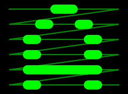
It turns out that we can encode every bit of information with 11 bits of the Barker sequence — a straight line for ones and an inverse for zeros. The elements of the Barker sequence are called chips . In practice, the coding goes like this:

The receiver can simply count the correlation of the Barker sequences (direct and inverse) and the input signal and determine from the peaks of the correlation function - where are the zeros in the input signal and where are the units
Modulation
In general - how to make a narrow-band noise-like information signal from a narrow-band information signal, and then restore it - we figured it out. Now let's talk a little about the ways of data transmission through the medium - the medium can be vacuum, air, optical fiber, wire, etc. In order to transmit a signal using radio waves, we need a carrier frequency, modulating it - we push our information onto the carrier. There are 3 main types of modulation - amplitude, frequency and phase.
It is possible to send our signal, ready for transmission, to a switch and simply switch on and off the transmission of the carrier - thereby modulating the amplitude
The advantages and disadvantages of amplitude modulation were considered in this article , so we will not dwell on it in detail here - at present, amplitude modulation is almost not used.
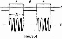
The next type of modulation is frequency , when the data signal controls the carrier frequency — either directly (VCO) or by switching between two different generators (a phase jump occurs)
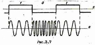
Here, too, have something to say, but some other time - otherwise the article will turn out too big.
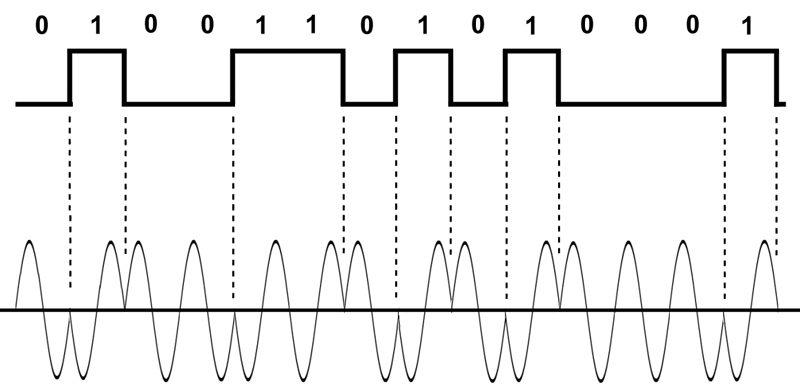
Phase modulation
It is easy to guess - here we encode information in the signal phase - for example, zero corresponds to zero phase shift, and one - to 180 degree shift - this encoding method is easy to implement technically - for example, multiplying the signal by 1 - we have zero phase shift, and multiplying by - 1 - 180 degree shift. This modulation is called Binary Phase Shift Key or BPSK.
What if we want to have more phase shifts? To begin, I will explain the logic of the engineers who came up with the following dances with a tambourine - you only have 2 control signals - 1 and -1 and with the help of them you need to encode an arbitrary number of phase shifts in the simplest way - you can of course put some super DAC and control the generated frequency directly but math offers us something better. Namely, this is the formula:

By the way - based on it, we made a transition from the spectra of sinusoids and cosine waves with zero phases to the spectrum of sinusoids with non-zero phases and phase spectrum - now we just do the inverse transformation.
The Quadrature Modulation is based on this.

- together with the carrier, we generate another signal, which is shifted relative to the carrier by 90 degrees, that is, is in quadrature with it . Now - by controlling the amplitude of each signal (In phase and Quadrature) - by multiplying by 1 or -1, and then summing up - we can get 4 possible phase shifts already.
Now we can encode 2 bits at a time. That is, the transfer rate is doubled. But the probability of error, too, will inevitably increase.
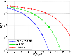
Similarly, a greater number of phase shifts can be obtained. Possible signal states are usually shown on a vector diagram or on a signal constellation plane.
Note that the sequence of binary words in the diagram is the Gray Code , which minimizes the probability of error. In addition - there is an additional shift of 45 degrees - this is done in order to reduce the parasitic amplitude modulation with phase jumps of 180 degrees
In practice, the synchronous method of transmission is not used - because there is a link to some initial phase, and over time an error occurs and the phase floats away, you need to constantly reinstall the initial phase - synchronize the receiver and transmitter. Therefore, the information carrier in real systems is not a phase, but a phase change — a differential signal transmission method allows one to get rid of synchronization. For example, each time zero appears, the phase makes a 180 degree jump (BPSK).
Then you can begin to talk about the intricacies of implementation - as always - in practice everything turns out to be more complicated than in theory, this article is more likely a small educational program for expanding horizons.
Source: https://habr.com/ru/post/192120/
All Articles