Everything you wanted to know about dynamic programming, but were afraid to ask
I was extremely surprised to find few articles about dynamic programming (hereinafter just dynamics) on Habré. It always seemed to me that this paradigm is quite widespread, including outside of programming contests. Therefore, I will try to close this gap with my article.
Perhaps the best description of the dynamics in one sentence that I have ever heard:
To successfully solve the problem of dynamics you need:
1) The state of the dynamics: the parameter (s) that uniquely set the subtask.
2) The values of the initial states.
3) State transitions: recalculation formula.
4) The procedure for recalculation.
5) The position of the answer to the problem: sometimes it is the sum or, for example, the maximum of the values of several states.
')
There are three recalculation procedures:
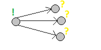
1) Direct order:
The states are sequentially recalculated based on those already counted.
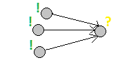
2) Reverse order:
All states that depend on the current state are updated.
3) Lazy dynamics:
Recursive memoized dynamic conversion function. This is something like a depth search in an acyclic state graph, where the edges are dependencies between them.
An elementary example: Fibonacci numbers . Status - the number number.
Direct order:
Reverse order:
Lazy dynamics:
All three options have the right to life. Each of them has its own scope, although it often intersects with others.
An example of one-dimensional dynamics is given above, in “recalculation order”, so I will immediately begin with multidimensional. It differs from the one-dimensional, as you may have guessed, the number of measurements, that is, the number of parameters in the state. Classification on this basis is usually based on the scheme “one-two-many” and is not very important, in fact.
The multidimensional dynamics are not very different from the one-dimensional, as you can see by looking at a couple of examples:
Previously, when the phones had buttons, their keyboards looked like this:

It is required to calculate how many different text messages to write multiplely using no more than
A chess knight stands in a cage

If you have never multiplied the matrices, but you want to understand this title, then you should read at least a wiki .
Suppose there is a task that we have already solved by dynamic programming, for example, the eternal Fibonacci numbers.
Let's reformulate it a bit. Suppose we have a vector from which we want to get a vector
  . Slightly open the formula:
  . You may notice that from the vector can get a vector
  by multiplying by some matrix, because in the final vector only folded variables from the first vector appear. This matrix is easy to derive, here it is:
  . Let's call it the transition matrix.
This means that if you take a vector and multiply it by the transition matrix
  in which
And now, why all this is necessary. Matrix multiplication has the property of associativity, that is, (but it does not have commutativity, which is surprising to me). This property gives us the right to do so:
  .
.
This is good because you can now apply the quick exponentiation method that works for . Total we were able to calculate the
And now an example is more serious:
We denote a sawtooth sequence of length

This is a class of dynamics in which the state is the subsection boundaries of an array. The point is to calculate the answers for subtasks based on all possible sub-segments of our array. Usually they are sorted in order of increasing length, and the recalculation is based, respectively, on shorter segments.
Here is the expanded condition . I will briefly retell it:
Define a compressed string:
1) A letter-only string is a concise string. Unclench it in itself.
2) A string that is the concatenation of two compressed strings
3) Line
Example:
It is necessary to find the length of the shortest compressed string unfolded into it by line
The state of dynamics parameter for subtrees is usually a vertex denoting a subtree in which this vertex is the root. To obtain the value of the current state, you usually need to know the results of all your children. Most often they implement it lazily - they just write a depth-first search from the root of the tree.
Given a hanging tree, in the leaves of which one-bit numbers are written -

It is required to find the minimum number of changes of logical operations in the internal vertices, such that the value in the root changes or report that this is impossible.
In dynamics over subsets, a mask of a given set usually enters the state. They are most often moved in the order of increasing the number of units in this mask and are recalculated, respectively, from the states that are smaller in inclusion. Usually used lazy dynamics, so as not to specifically think about the traversal order, which sometimes is not quite trivial.
A weighted (non-negative, edge weight) graph
Classical problems that are solved by the dynamics of the profile, are the tasks on the paving of the field by some kind of figures. Moreover, different things may be asked, for example, the number of ways of paving or paving with a minimum number of pieces.
These tasks can be solved by exhaustive search. where
where  .
.
A profile is

Almost always the state is the profile and where the profile is. A transition increases this location by one. It is possible to find out whether it is possible to go from one profile to another within a linear time of the profile size. This can be checked each time during the recalculation, but it can also be assumed. We will presuppose a two-dimensional array of
Find the number of ways to tile an
This is a very strong optimization of the dynamics of the profile. Here the profile is not only a mask, but also a place of a break. It looks like this:

Now, after adding a break in the profile, you can move to the next state by adding just one figure covering the left break cell. That is, by increasing the number of states before
  . Asymptotics improved with before
  .
.
Transitions in dynamics along a broken profile using the example of a task about tiling with dominoes (Example No. 8):

Sometimes it happens that simply knowing some characteristic of a better answer is not enough. For example, in the “Packing a string” task (example No. 4), we end up with only the length of the shortest compressed string, but, most likely, we need not its length, but the string itself. In this case, you need to restore the answer.
Each task has its own way of recovering the answer, but the most common ones are:
Often, in dynamics, one can encounter a task in which a state requires not a very large number of other states to be counted. For example, when calculating Fibonacci numbers, we use only the last two, and we will never turn to the previous ones. So, you can forget about them, that is, do not store in memory. Sometimes this improves the asymptotic memory estimate. This technique can be used in examples No. 1, No. 2, No. 3 (in the solution without a transition matrix), No. 7 and No. 8. True, this can not be used in any way, if the bypass order is a lazy speaker.
Sometimes it happens that you can improve the asymptotic time using some kind of data structure. For example, in the Dijkstra algorithm, you can use the priority queue to change the asymptotic time.
In solutions, dynamics necessarily include a state — parameters that uniquely define a subtask, but this state is not necessarily the only one. .
1) :
2) :
3) :
4) : ,
5) —
: , :
, :  . :
. :  .
.
1) . dp[n][k] —
2) :
3) :
, . ( ) :
, :

.
, — . — , , — : .
4) : ,
, ,  . , —
. , —  (
(  .
.
5) —
: .
, ( ), ( darnley ).
, - ! — , .
# Python The basics
Perhaps the best description of the dynamics in one sentence that I have ever heard:
Dynamic programming is when we have a task that is not clear how to solve, and we break it down into smaller tasks that are also not clear how to solve. (c) A. Kumok.
To successfully solve the problem of dynamics you need:
1) The state of the dynamics: the parameter (s) that uniquely set the subtask.
2) The values of the initial states.
3) State transitions: recalculation formula.
4) The procedure for recalculation.
5) The position of the answer to the problem: sometimes it is the sum or, for example, the maximum of the values of several states.
')
Recalculation procedure
There are three recalculation procedures:
1) Direct order:
The states are sequentially recalculated based on those already counted.
2) Reverse order:
All states that depend on the current state are updated.
3) Lazy dynamics:
Recursive memoized dynamic conversion function. This is something like a depth search in an acyclic state graph, where the edges are dependencies between them.
An elementary example: Fibonacci numbers . Status - the number number.
Direct order:
fib[1] = 1 # fib[2] = 1 # for i in range(3, n + 1): fib[i] = fib[i - 1] + fib[i - 2] # i Reverse order:
fib[1] = 1 # for i in range(1, n): fib[i + 1] += fib[i] # i + 1 fib[i + 2] += fib[i] # i + 2 Lazy dynamics:
def get_fib(i): if (i <= 2): # return 1 if (fib[i] != -1): # return fib[i] fib[i] = get_fib(i - 1) + get_fib(i - 2) # return fib[i] All three options have the right to life. Each of them has its own scope, although it often intersects with others.
Multidimensional dynamics
An example of one-dimensional dynamics is given above, in “recalculation order”, so I will immediately begin with multidimensional. It differs from the one-dimensional, as you may have guessed, the number of measurements, that is, the number of parameters in the state. Classification on this basis is usually based on the scheme “one-two-many” and is not very important, in fact.
The multidimensional dynamics are not very different from the one-dimensional, as you can see by looking at a couple of examples:
Example # 1: Number of SMS
Previously, when the phones had buttons, their keyboards looked like this:
It is required to calculate how many different text messages to write multiplely using no more than
k clicks on such a keyboard.Decision
1) The state of the dynamics:
2) Initial state: there is one message of length zero, using zero presses - empty.
3) Conversion formulas: there are eight letters each, for which you need to write one, two and three clicks, as well as two letters that require 4 clicks.
Direct conversion:
4) The procedure for recalculation:
If we write using the direct method, then we need to think separately about going beyond the dynamics, for example, when we refer to
When using the reverse recalculation, everything is simpler: we always turn forward, so we will not leave the negative elements.
5) The answer is the sum of all states.
UPD:
Unfortunately, I made a mistake - the problem can be solved one-dimensional, simply by removing the length of the message
1) State:
2) Initial state:
3) Conversion formula:
5) The answer is the sum of all states.
dp[n][m] - the number of different messages of length n , using m clicks.2) Initial state: there is one message of length zero, using zero presses - empty.
3) Conversion formulas: there are eight letters each, for which you need to write one, two and three clicks, as well as two letters that require 4 clicks.
Direct conversion:
dp[n][m] = (dp[n - 1][m - 1] + dp[n - 1][m - 2] + dp[n - 1][m - 3]) * 8 + dp[n - 1][m - 4] * 2 Reverse conversion: dp[n + 1][m + 1] += dp[n][m] * 8 dp[n + 1][m + 2] += dp[n][m] * 8 dp[n + 1][m + 3] += dp[n][m] * 8 dp[n + 1][m + 4] += dp[n][m] * 2 4) The procedure for recalculation:
If we write using the direct method, then we need to think separately about going beyond the dynamics, for example, when we refer to
dp[n - 1][m - 4] , which may not exist for small m . To circumvent this, you can either put checks in terms of recalculation or write neutral elements there (which do not change the answer).When using the reverse recalculation, everything is simpler: we always turn forward, so we will not leave the negative elements.
5) The answer is the sum of all states.
UPD:
Unfortunately, I made a mistake - the problem can be solved one-dimensional, simply by removing the length of the message
n from the state.1) State:
dp[m] - the number of different posts that can be typed in m taps.2) Initial state:
dp[0] = 1 .3) Conversion formula:
dp[m] = (dp[m - 1] + dp[m - 2] + dp[m - 3]) * 8 + dp[m - 4] * 2 4) Order: all three options can be used.5) The answer is the sum of all states.
Example 2: Horse
A chess knight stands in a cage
(1, 1) on an N x M size board. It is required to count the number of ways to get to the cell (N, M) moving in four types of steps:Decision
1) The state of the dynamics:
2) Initial value: In the cell
3) Conversion formula:
For direct order:
4) And now the most interesting thing in this problem: order. Here you can not just go and walk through the rows or columns. Because otherwise, we will refer to the not yet recalculated states in the direct order, and we will take more unfinished states in the opposite approach.
There are two ways:
1) Come up with a good detour.
2) Launch lazy dynamics, let them figure it out.
If you are too lazy to think, we are launching lazy dynamics, she will do an excellent job with the task.
If not laziness, then you can think of a detour like this:

This procedure ensures that all the cells required at each step are processed during the direct walk, and the current state is processed at the reverse.
5) The answer simply lies in
dp[i][j] - the number of ways to get to (i, j) .2) Initial value: In the cell
(1, 1) can be reached in one way - do nothing.3) Conversion formula:
For direct order:
dp[i][j] = dp[i - 2][j - 1] + dp[i - 2][j + 1] + dp[i - 1][j - 2] + dp[i + 1][j - 2] For reverse order: dp[i + 1][j + 2] += dp[i][j] dp[i + 2][j + 1] += dp[i][j] dp[i - 1][j + 2] += dp[i][j] dp[i + 2][j - 1] += dp[i][j] 4) And now the most interesting thing in this problem: order. Here you can not just go and walk through the rows or columns. Because otherwise, we will refer to the not yet recalculated states in the direct order, and we will take more unfinished states in the opposite approach.
There are two ways:
1) Come up with a good detour.
2) Launch lazy dynamics, let them figure it out.
If you are too lazy to think, we are launching lazy dynamics, she will do an excellent job with the task.
If not laziness, then you can think of a detour like this:
This procedure ensures that all the cells required at each step are processed during the direct walk, and the current state is processed at the reverse.
5) The answer simply lies in
dp[n][m] .Dynamics and transition matrix
If you have never multiplied the matrices, but you want to understand this title, then you should read at least a wiki .
Suppose there is a task that we have already solved by dynamic programming, for example, the eternal Fibonacci numbers.
Let's reformulate it a bit. Suppose we have a vector
. Slightly open the formula: . You may notice that from the vector by multiplying by some matrix, because in the final vector only folded variables from the first vector appear. This matrix is easy to derive, here it is: . Let's call it the transition matrix.This means that if you take a vector
and multiply it by the transition matrix n - 1 times, then we get the vector in which fib[n] lies - the answer to the problem.And now, why all this is necessary. Matrix multiplication has the property of associativity, that is,
(but it does not have commutativity, which is surprising to me). This property gives us the right to do so: .This is good because you can now apply the quick exponentiation method that works for
. Total we were able to calculate the N th Fibonacci number for the logarithm of arithmetic operations.And now an example is more serious:
Example 3: sawtooth sequence
We denote a sawtooth sequence of length
N as a sequence in which the condition is satisfied for each non-extreme element: it is either less than or both of its neighbors or more. It is required to count the number of sawtooth sequences from digits of length N It looks something like this:Decision
To begin with, a solution without a transition matrix:
1) The state of the dynamics:
2) Initial values:
5) The answer is the sum of
Now we need to come up with an initial vector and a transition matrix. The vector seems to be invented quickly: all the states that indicate the length of the sequence
1) The state of the dynamics:
dp[n][last][less] - the number of sawtooth sequences of length n , ending in the digit last . And if less == 0 , then the last digit is less than the last but one, and if less == 1 , it means more.2) Initial values:
for last in range(10): dp[2][last][0] = 9 - last dp[2][last][1] = last 3) Recalculation of the dynamics: for prev in range(10): if prev > last: dp[n][last][0] += dp[n - 1][prev][1] if prev < last: dp[n][last][1] += dp[n - 1][pref][0] 4) Recalculation order: we always refer to the previous length, so just a pair of nested for 's.5) The answer is the sum of
dp[N][0..9][0..1] .Now we need to come up with an initial vector and a transition matrix. The vector seems to be invented quickly: all the states that indicate the length of the sequence
N Well, the transition matrix is displayed, looking at the recalculation formulas.Vector and transition matrix
Dynamics by subseries
This is a class of dynamics in which the state is the subsection boundaries of an array. The point is to calculate the answers for subtasks based on all possible sub-segments of our array. Usually they are sorted in order of increasing length, and the recalculation is based, respectively, on shorter segments.
Example 4: Packing a string
Here is the expanded condition . I will briefly retell it:
Define a compressed string:
1) A letter-only string is a concise string. Unclench it in itself.
2) A string that is the concatenation of two compressed strings
A and B It expands into the concatenation of the expanded A and B lines.3) Line
D(X) , where D is an integer greater than 1 , and X is a compressed string. It expands to the concatenation of D strings expanded from XExample:
“3(2(A)2(B))C” expanded in “AABBAABBAABBC” .It is necessary to find the length of the shortest compressed string unfolded into it by line
s .Decision
This problem is being solved, as you probably already guessed, by sub-cutting dynamics.
1) The state of the dynamics:
2) Initial states: all substrings of length one can be compressed only in themselves.
3) Recalculation of the dynamics:
The best answer has some sort of final compression operation: either it is just a string of capital letters, or it is a concatenation of two lines, or compression itself. So let's go through all the options and choose the best.
5) The answer lies in
1) The state of the dynamics:
d[l][r] - compressed string of minimum length, unclamping into a string s[l:r]2) Initial states: all substrings of length one can be compressed only in themselves.
3) Recalculation of the dynamics:
The best answer has some sort of final compression operation: either it is just a string of capital letters, or it is a concatenation of two lines, or compression itself. So let's go through all the options and choose the best.
dp_len = r - l dp[l][r] = dp_len # - . for i in range(l + 1, r): dp[l][r] = min(dp[l][r], dp[l][i] + dp[i][r]) # for cnt in range(2, dp_len): if (dp_len % cnt == 0): # , good = True for j in range(1, (dp_len / cnt) + 1): # , cnt good &= s[l:l + dp_len / cnt] == s[l + (dp_len / cnt) * j:l + (dp_len / cnt) * (j + 1)] if good: # cnt dp[l][r] = min(dp[l][r], len(str(cnt)) + 1 + dp[l][l + dp_len / cnt] + 1) 4) The order of conversion: direct ascending the length of the substring or lazy dynamics.5) The answer lies in
d[0][len(s)] .Example 5: Oaks
Subtree dynamics
The state of dynamics parameter for subtrees is usually a vertex denoting a subtree in which this vertex is the root. To obtain the value of the current state, you usually need to know the results of all your children. Most often they implement it lazily - they just write a depth-first search from the root of the tree.
Example 6: Logical tree
Given a hanging tree, in the leaves of which one-bit numbers are written -
0 or 1 . All internal vertices also contain numbers, but according to the following rule: for each vertex one of the logical operations is chosen: “AND” or “OR”. If it is “AND”, then the value of the vertex is the logical “AND” of the values of all its children. If "OR", then the value of the vertex is the logical "OR" of the values of all its children.It is required to find the minimum number of changes of logical operations in the internal vertices, such that the value in the root changes or report that this is impossible.
Decision
1) The state of the dynamics:
2) Initial values: for leaves, it is obvious that its value can be obtained for zero changes, but it is impossible to change the value, that is, it is possible, but only for
3) Conversion formula:
If at this vertex is already the value of
If the operation "And" and you need to get "0", then the answer is the minimum of the values of
If the operation "And" and you need to get "1", then the answer is the sum of all values of
If the operation is "OR" and you need to get "0", then the answer is the sum of all
If the operation is "OR" and you need to get "1", then the answer is the minimum of the values
4) The order of conversion: the easiest to implement is lazy - in the form of a search into the depth of the root.
5) The answer is
d[v][x] - the number of operations required to obtain the value of x at the vertex v . If this is not possible, then the state value is +inf .2) Initial values: for leaves, it is obvious that its value can be obtained for zero changes, but it is impossible to change the value, that is, it is possible, but only for
+inf operations.3) Conversion formula:
If at this vertex is already the value of
x , then zero. If not, then there are two options: change the operation in the current vertex or not. For both you need to find the best option and choose the best.If the operation "And" and you need to get "0", then the answer is the minimum of the values of
d[i][0] , where i is the son of v .If the operation "And" and you need to get "1", then the answer is the sum of all values of
d[i][1] , where i is the son of v .If the operation is "OR" and you need to get "0", then the answer is the sum of all
d[i][0] values, where i is the son of v .If the operation is "OR" and you need to get "1", then the answer is the minimum of the values
d[i][1] , where i is the son of v .4) The order of conversion: the easiest to implement is lazy - in the form of a search into the depth of the root.
5) The answer is
d[root][value[root] xor 1] .The dynamics of the subsets
In dynamics over subsets, a mask of a given set usually enters the state. They are most often moved in the order of increasing the number of units in this mask and are recalculated, respectively, from the states that are smaller in inclusion. Usually used lazy dynamics, so as not to specifically think about the traversal order, which sometimes is not quite trivial.
Example # 7: Hamiltonian cycle of minimum weight, or the traveling salesman problem
A weighted (non-negative, edge weight) graph
G size N . Find the Hamiltonian cycle (the cycle passing through all vertices without self-intersections) of the minimum weight.Decision
Since we are looking for a cycle passing through all the vertices, we can choose any one as the “initial” vertex. Let it be the vertex with the number
1) The state of the dynamics:
2) Initial values:
3) The recalculation formula: If the
4) Recalculation order: the easiest and most convenient way is to write lazy dynamics, but you can turn around and write through the masks in order of increasing the number of single bits in it.
5) The answer lies in
0 .1) The state of the dynamics:
dp[mask][v] - the path of the minimum weight from the vertex 0 to the vertex v , passing through all the vertices lying in the mask and only along them.2) Initial values:
dp[1][0] = 0 , all other states initially - +inf .3) The recalculation formula: If the
i -th bit in mask is 1 and there is an edge from i to v , then: dp[mask][v] = min(dp[mask][v], dp[mask - (1 << i)][i] + w[i][v]) Where w[i][v] is the weight of the edge from i to v .4) Recalculation order: the easiest and most convenient way is to write lazy dynamics, but you can turn around and write through the masks in order of increasing the number of single bits in it.
5) The answer lies in
d[(1 << N) - 1][0] .Profile Dynamics
Classical problems that are solved by the dynamics of the profile, are the tasks on the paving of the field by some kind of figures. Moreover, different things may be asked, for example, the number of ways of paving or paving with a minimum number of pieces.
These tasks can be solved by exhaustive search.
where a is the number of options for tiling a single cell. The dynamics of the profile optimizes the time for one of the dimensions to linear, leaving only the coefficient in the exponent. It turns out something like this: A profile is
k (often single) columns, which are the boundary between the already tiled part and the not yet tiled part. This border is only partially filled. It is often part of the state of the dynamics.Almost always the state is the profile and where the profile is. A transition increases this location by one. It is possible to find out whether it is possible to go from one profile to another within a linear time of the profile size. This can be checked each time during the recalculation, but it can also be assumed. We will presuppose a two-dimensional array of
can[mask][next_mask] - can we move from one mask to another by putting several figures, increasing the position of the profile by one. If it is presumed, then it takes less time to complete, and more memory.Example 8: Dominoing
Find the number of ways to tile an
N x M table using dominoes with dimensions of 1 x 2 and 2 x 1 .Decision
Here the profile is one column. It is convenient to store it in the form of a binary mask:  .
.
0) Pre-submission (optional): enumerate all pairs of profiles and check that one can go from one to another. In this problem, it is verified as follows:
If in the first profile in the next place is
If in the first profile in the next place is
If
Examples of transitions (from the top profile you can go to the bottom and only to them):

After that, save everything to the array
1) The state of the dynamics:
2) Initial state:
3) Conversion formula:
4) Bypass order - in order of increasing
5) The answer lies in dp [pos] [0].
The resulting asymptotics is .
.
0 - not tiled column cell, 1 - tiled. That is, the total profiles .0) Pre-submission (optional): enumerate all pairs of profiles and check that one can go from one to another. In this problem, it is verified as follows:
If in the first profile in the next place is
1 , then in the second one must necessarily be 0 , since we will not be able to tile this cell with any figurine.If in the first profile in the next place is
0 , then there are two options - or in the second 0 or 1 .If
0 , it means that we are obliged to put a vertical domino, which means the next cell can be considered as 1 . If 1 , then we put a vertical domino and go to the next cell.Examples of transitions (from the top profile you can go to the bottom and only to them):
After that, save everything to the array
can[mask][next_mask] - 1 , if you can go, 0 - if you can not.1) The state of the dynamics:
dp[pos][mask] - the number of complete tilings of the first pos - 1 columns with the mask profile.2) Initial state:
dp[0][0] = 1 - the left field boundary is a straight wall.3) Conversion formula:
dp[pos][mask] += dp[pos - 1][next_mask] * can[mask][next_mask] 4) Bypass order - in order of increasing
pos .5) The answer lies in dp [pos] [0].
The resulting asymptotics is
.The dynamics of the broken profile
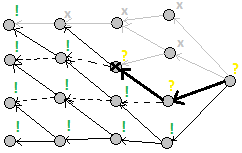
This is a very strong optimization of the dynamics of the profile. Here the profile is not only a mask, but also a place of a break. It looks like this:
Now, after adding a break in the profile, you can move to the next state by adding just one figure covering the left break cell. That is, by increasing the number of states
N times (remember, where the break is) we reduced the number of transitions from one state to another with before . Asymptotics improved with .Transitions in dynamics along a broken profile using the example of a task about tiling with dominoes (Example No. 8):
Recovery response
Sometimes it happens that simply knowing some characteristic of a better answer is not enough. For example, in the “Packing a string” task (example No. 4), we end up with only the length of the shortest compressed string, but, most likely, we need not its length, but the string itself. In this case, you need to restore the answer.
Each task has its own way of recovering the answer, but the most common ones are:
- Next to the value of the state of the dynamics store the full response to the subtask. If the answer is something big, then you may need too much memory, so if you can use another method, they usually do it.
- Restore the answer, knowing the ancestor (s) of this state. Often, you can restore the answer, knowing only how it was received. In the very "Packing line" you can save the answer to store only the last action view and the state from which it was obtained.
- There is a way that does not use additional memory at all - after recalculating the dynamics, go from the end to the best way and form an answer along the way.
Small optimizations
Memory
Often, in dynamics, one can encounter a task in which a state requires not a very large number of other states to be counted. For example, when calculating Fibonacci numbers, we use only the last two, and we will never turn to the previous ones. So, you can forget about them, that is, do not store in memory. Sometimes this improves the asymptotic memory estimate. This technique can be used in examples No. 1, No. 2, No. 3 (in the solution without a transition matrix), No. 7 and No. 8. True, this can not be used in any way, if the bypass order is a lazy speaker.
Time
Sometimes it happens that you can improve the asymptotic time using some kind of data structure. For example, in the Dijkstra algorithm, you can use the priority queue to change the asymptotic time.
State replacement
In solutions, dynamics necessarily include a state — parameters that uniquely define a subtask, but this state is not necessarily the only one. .
№9:
N . , N = 7 , 5 :- 7
- 3 + 4
- 2 + 5
- 1 + 7
- 1 + 2 + 4
№1:
1) :
dp[n][k] — n , k . k , , .2) :
dp[1][1] = 1 , dp[1][i] = 0 .3) :
for last_summand in range(1, k + 1): dp[n][k] += dp[n - last_summand][last_summand] 4) : ,
n .5) —
dp[N][1..N] .:
. : .№2:
1) . dp[n][k] —
n k . , .2) :
dp[1][1] = 1 , dp[1][i] = 0 .3) :
dp[n][k] = dp[n - k][k] + dp[n - k][k - 1] , . ( ) :
1.1.1.
, :
.
, — . — , , — : .
4) : ,
n .,
. , — k N , ( 1 k ). , 5) —
dp[N][1..k_max] .:
Conclusion
, ( ), ( darnley ).
, - ! — , .
Source: https://habr.com/ru/post/191498/
All Articles