Why is not everything normal with normal distribution

The normal distribution (Gaussian distribution) has always played a central role in the theory of probability, since it very often occurs as a result of the influence of many factors, the contribution of any one of which is negligible. The Central Limit Theorem (CLT), is used in virtually all applied sciences, making the statistical apparatus universal. However, there are very frequent cases where its use is impossible, and researchers are trying in every possible way to organize the fitting of results to Gaussians. I will now tell you about the alternative approach in the case of influence on the distribution of many factors.

A brief history of the CLT. While still alive Newton, Abraham de Moivre proved a theorem on the convergence of a centered and normalized number of observations of an event in a series of independent tests to a normal distribution. Throughout the 19th and early 20th centuries, this theorem served as a scientific model for generalizations. Laplace proved the case of a uniform distribution, Poisson proved a local theorem for a case with different probabilities. Poincare, Legendre, and Gauss developed a rich theory of observation errors and the least squares method, based on the convergence of errors to the normal distribution. Chebyshev proved an even stronger theorem for the sum of random variables by developing a method of moments for a campaign. Lyapunov in 1900, relying on Chebyshev and Markov, proved the CLT in its current form, but only with the existence of third-order moments. And only in 1934, Feller put an end to it, showing that the existence of second-order moments is both a necessary and sufficient condition.

The CLT can be formulated as follows: if random variables are independent, equally distributed and have a finite variance other than zero, then the sums (centered and normalized) of these quantities converge to the normal law. It is in this form that this theorem is taught in universities, and it is so often used by observers and researchers who are not professional in mathematics. What is wrong with her? In fact, the theorem is perfectly applied in the areas that Gauss, Poincaré, Chebyshev, and other geniuses of the 19th century worked on, namely: the theory of observation errors, statistical physics, OLS, demographic research, and maybe something else. But scientists who lack originality for discoveries are engaged in generalizations and want to apply this theorem to everything, or simply drag the normal distribution by the ears, where it simply cannot be. Want examples, I have them.
')
IQ of IQ. Initially implies that people's intelligence is distributed normally. Conduct a test that is pre-compiled in such a way that it does not take into account outstanding abilities, but is taken into account separately with the same fractional factors: logical thinking, mental design, computational abilities, abstract thinking and something else. The ability to solve problems inaccessible to the majority, or passing a test in ultra-fast time is not taken into account, and passing the test earlier increases the result (but not the intellect) in the future. And then the philistines and believe that "no one is twice as smart as they can be," "let us take and divide from the clever men."

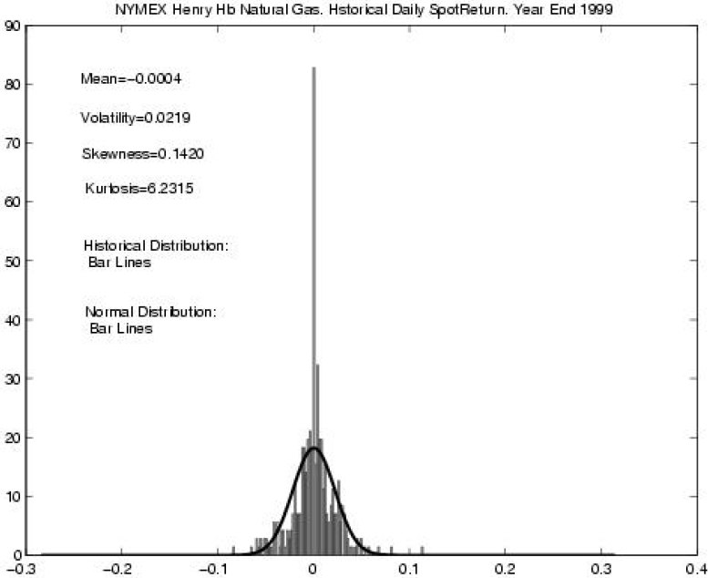
The second example: changes in financial performance. Studies of changes in stock prices, currency quotes, commodity options require the use of mathematical statistics, and it is especially important not to make a mistake with the type of distribution. Case in point: in 1997, the Nobel Prize in economics was paid for proposing a Black - Scholes model based on the assumption that the distribution of stock indicators was normal (the so-called white noise). At the same time, the authors clearly stated that this model needs to be refined, but all that the majority of further researchers decided on was simply to add the Poisson distribution to the normal distribution. Here, obviously, there will be inaccuracies in the study of long time series, since the Poisson distribution satisfies the CLT too well, and already with 20 terms it is indistinguishable from the normal distribution. Look at the picture below (and it is from a very serious economic journal); it shows that, despite the rather large number of observations and obvious distortions, it is assumed that the distribution is normal.



It is quite obvious that the normal distribution of wages among the population of the city, the size of files on disk, the population of cities and countries will not be normal.

The common feature of the distributions of these examples is the presence of the so-called “heavy tail”, that is, values ​​that lie far from the mean, and noticeable asymmetry, as a rule, is right. Let us consider what else besides the normal distribution could be. Let's start with the Poisson mentioned earlier: it has a tail, but we want the law to be repeated for the aggregate of groups, in each of which it is observed (count the size of files by enterprise, salary for several cities) or scale (randomly increase or decrease the model interval Black-Scholes), as observations show, tails and asymmetry do not disappear, but the Poisson distribution, according to the CLT, should become normal. For the same reasons, Erlang, beta, logonormal, and all other variances will not work. It remains only to cut off the Pareto distribution, but it is not suitable due to the coincidence of the mode with the minimum value, which is almost not found in the analysis of sample data.

Distributions possessing the necessary properties exist and are called stable distributions. Their history is also very interesting, and the main theorem was proved a year after Feller’s work, in 1935, by the joint efforts of the French mathematician Paul Levy and the Soviet mathematician A.Ya. Khinchin The CLT was generalized, the condition for the existence of dispersion was removed from it. Unlike the normal, neither the density nor the distribution function of stable random variables are expressed (with rare exceptions, which are described below), all that is known about them is a characteristic function (the inverse Fourier transform of the distribution density, but to understand the essence it is possible and not know).
So, the theorem: if the random variables are independent, equally distributed, then the sums of these quantities converge to a stable law.

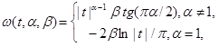
Now the definition. The random variable X will be stable if and only if the logarithm of its characteristic function present in the form:





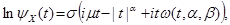
Where .

In fact, there is nothing much difficult here, just to explain the meaning of the four parameters. Parameters sigma and mu - the usual scale and offset, as in the normal distribution, mu will be equal to the expectation, if it is, and it is, when alpha is more than one. The beta parameter is the asymmetry, when it is equal to zero, the distribution is symmetrical. But alpha is a characteristic parameter, it means what order the moments of the quantity exist, the closer it is to two, the more the distribution is similar to the normal one, when equal to two, the distribution becomes normal, and only in this case does it have moments of higher orders, also in the case normal distribution, asymmetry degenerates. In the case when alpha is one and beta is zero, the Cauchy distribution is obtained, and in the case when alpha is half and beta unit is the Levi distribution, in other cases there is no representation in quadratures for the distribution density of such quantities.
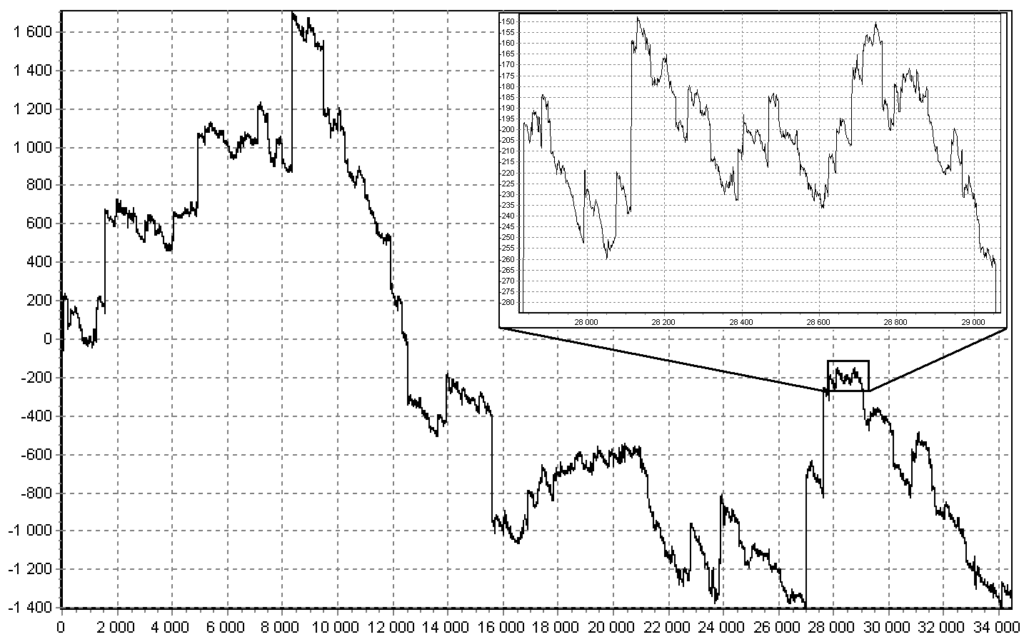
In the 20th century, a rich theory of stable quantities and processes was developed (called Levi processes), their relationship with fractional integrals was shown, various methods of parameterization and modeling were introduced, parameters were estimated in several ways, and consistency and stability of estimates were shown. Look at the picture, on it is a simulated trajectory of the Levy process with a fragment enlarged 15 times.



Being engaged in such processes and their application in finance, Benoit Mandelbrot invented fractals. However, not everywhere was so good. The second half of the 20th century passed under the general trend of applied and cybernetic sciences, which meant a crisis of pure mathematics, everyone wanted to produce, but did not want to think, the humanities with their journalism occupied the mathematical realms. Example: the book "Fifty entertaining probabilistic problems with solutions" by American Mosteller, problem number 11:



The author's solution to this problem is simply a defeat of common sense:


The same situation with the 25 task, where there are THREE contradictory answers.

But back to sustainable distributions. In the remainder of this article I will try to show that there should be no additional difficulties when working with them. Namely, there are numerical and statistical methods that allow estimating parameters, calculating the distribution function and simulating them, that is, working the same way as with any other distribution.

Simulation of stable random variables. Since everything is known in comparison, I first recall the most convenient, in terms of calculations, the method of generating a normal value (the Box – Muller method): - basic random variables (uniformly distributed on [0, 1) and independent), then by the ratio

get the standard normal value.

Now let us set in advance alpha and beta, let V and W , independent random variables: V evenly distributed on , W is exponentially distributed with parameter 1, we define and , then by the ratio:

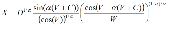
we obtain a stable random variable for which the mu is zero and sigma is one. This is the so-called standard stable value, which, for the general case (with alpha not equal to one), is simply enough to multiply by scale and add offset. Yes, the ratio is more complicated, but it is still simple enough to use even in spreadsheets ( Reference ). The figures below show the trajectories of modeling the Black - Scholes model, first for the normal and then for the sustainable process.






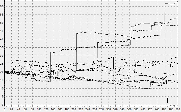
You can believe the price chart on the stock exchanges is more like the second.

Estimation of parameters of sustainable distribution. As it is rather difficult to insert formulas in Habré, I will simply leave a link to the article, where various methods for estimating parameters are analyzed in detail, or to my article in Russian, where only two methods are given. You can also find a wonderful book that contains the whole theory on stable random variables and their applications (Zolotarev V., Uchaikin V. Stable Distributions and their Applications. VSP. M.: 1999.), or its purely Russian version (Zolotarev V .M. Stable one-dimensional distributions. - M .: Nauka, Main editors of physical and mathematical literature, 1983. - 304 p. These books also contain methods for calculating the density and distribution function.

As a conclusion, I can only recommend, when analyzing statistical data, when there is asymmetry or values ​​that are much higher than expected, ask yourself: “is the distribution law correct?” And “is everything normal with normal distribution?”.