Fluid Dynamics Simulation: Lattice Boltzmann Method

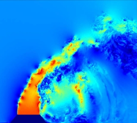
Simulation of a volcanic eruption
using Lattice Boltzmann Method. (c) Source

In this article I will talk about the numerical method for modeling hydrodynamics Lattice Boltzmann Method , LBM. In Russian, the Boltzmann method of lattice equations. It is superior to other well-known methods (for example, the finite element method ) in ease of parallelization, the ability to simulate multiphase flows, modeling flows in porous media. In addition, the computational algorithm contains only the simplest arithmetic operations. The method is very new, the first commercial products based on it began to appear around 2010.

On Habré has already been a series of articles on the physics of fluid, and this article may be its logical continuation. It is written in such a way as to be useful to people who know hydrodynamics and modeling methods well, and understandable to beginners in this area (for example, people with education software engineer). Of course, in this regard, many things will be too detailed for experts, and some will not have enough space. The article was quite large, but I would not want to break it into several parts.

Why is all this necessary? More precisely, in which branches it is necessary to model hydrodynamics:

aircraft, rocket, automotive (body characteristics, engine performance, nozzles)
industrial chemistry (separation of substances, chemical reactors)
meteorology, geology (fluid flows through porous media, sandstones, dams)
other engineering industries (wind power)
medicine (blood flow, lymph)

The article will include the following sections:

Physics Review - High-level overview of basic equations needed
The main idea — the description of the basic principle of the algorithm
Technical details — a more detailed explanation of the initial equations, the derivation of a computational scheme
- Navier-Stokes equation
- Boltzmann equation
- Discrete boltzmann equation
- Illustration of computational scheme
- Spatial lattices
- Equilibrium distribution functions
- Incompressibility
- Viscosity and reynolds number
- Once again all together
miscellanea
- Additions to the algorithm
- Underwater rocks
- Existing solutions
- What to read

Physics review

Hydro and aerodynamics are macroscopically described by the Navier-Stokes equation . It shows what the pressure, density and velocity of the fluid will be at each point in space at each moment in time — depending on the initial and boundary conditions and environmental parameters.
')
On the other hand, for rarefied gases, the Boltzmann equation is true, which describes how the density of the particle velocity distribution varies at each point in space with time. If we integrate the distribution of particles over the velocities at a given point, we can obtain the density and macroscopic velocity at a given point. In other words, macroscopically, the Boltzmann equation is equivalent to the Navier-Stokes equation.

main idea

Despite the fact that for dense liquids, the Boltzmann equation is not applicable, if we learn to model it, we can also model the Navier-Stokes equation for these fluids. That is, we thereby replace the underlying level of abstractions (microscopic equation for dense liquids) with a physically incorrect implementation (microscopic equation for rarefied gases), but so that the upper level (the macroscopic Navier-Stokes equation) is described correctly.

The situation is illustrated in the picture below.
Lattice Boltzmann Method Idea

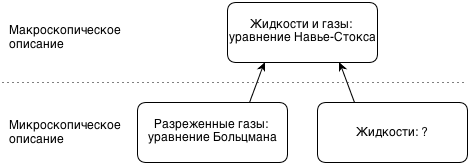
The question mark in it symbolizes the fact that I do not know which equation describes the behavior of dense liquids at the microscopic level. Sometimes, instead of “microscopic,” they say “mesoscopic” —in the sense that a microscopic description is a description of the behavior of individual atoms and molecules, and the Boltzmann equation describes flows of molecules.

Since the computer does not know how to work with continuous values, we need to discretize the Boltzmann equation: by time, by spatial coordinates (we get spatial nodes for modeling) and by possible directions of particles in each spatial node. Directions are chosen in a special way, and always point to some neighboring nodes.

Technical details

This large section contains a more detailed explanation of the initial equations and the derivation of a computational scheme. Really important equations should be clear to all readers with technical education (the basics of linear algebra, integral calculus are required). Those equations that are incomprehensible, most likely, are not important (they are those where there is nabla ). Vectors are indicated in bold.

Navier-Stokes equation

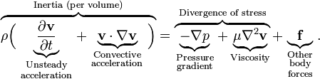
A variant of the equation for the macroscopic dynamics of incompressible liquids and gases is as follows:
Navier-Stokes equation

(one)

here v is the flow velocity, ρ is the density of the fluid, p is the pressure in the fluid, f is the external forces (for example, gravity).

If you do not know what inverted triangles and partial derivatives are — do not worry, we will not need them later, and the computational algorithm contains only the simplest arithmetic operations.

A detailed conclusion and the physical meaning can be studied on Wikipedia and Habré , but I will give the main idea here.

Mentally allocate a certain small volume in a liquid and follow its movement. The acceleration acting on a given volume of fluid is determined by (i) the pressures of the left, right, top, bottom, etc. (besides, they partially compensate each other), (ii) by the action of internal friction forces in a liquid (iii) by external forces. On the other hand, the acceleration can be expressed in terms of the velocity difference at the initial moment of time at the initial point and at some next moment in time at the new point where the fluid volume will be.

If we now substitute these values into the Newton equation F = ma, after some simple transformations, we get the equation above. On the left is ma, on the right — F.

Boltzmann equation

This equation operates on the function of the probability density distribution of particles in terms of coordinates and velocities, f (r, v, t). The value of f (x, y, z, v _x , v _y , v _z , t) dx dy dz dv _x dv _y dv _z shows what proportion of particles at time t is in a cube from x to x + dx, from y to y + dy, from z to z + dz with speeds in the range from v _x to v _x + dv _x , from v _y to v _y + dv _y , from v _z to v _z + dv _z . It can also be written as f (r, v, t) d ^ 3r d ^ 3v

.

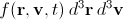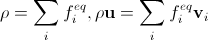
This function is usually normalized to the mass of gas in the system under study, therefore the macroscopic gas density at each point is defined as the sum (integral) of the probability density at a given point over all possible values of velocity,
Density

. (2)
Similarly, macroscopic speed can be determined by
Velocity

. (3)

The basic idea for deriving an equation is similar to the derivation of the Navier-Stokes equation. Let's mentally select at a given time in a given small volume a bundle of molecules flying in a given direction (more precisely, a narrow cone of directions). After a short period of time dt, they will be at the next point (due to the presence of speed), their speed itself will change due to the acceleration of molecules by external forces. In addition, on this segment of the path, some molecules will collide with others, change their speed, and we can no longer include them in the original beam. On the other hand, as a result of collisions of molecules in the same volume, flying in the other direction, some of them will acquire the desired direction of speed, and we will add them to the beam.

This can be written in the following form:
$Boltzmann derivation, f \ left (\ mathbf {r} + \ mathbf {v} dt, \ mathbf {v} + \ frac {\ mathbf {F}} {m} dt, t + dt \ right) \, d ^ 3 \ mathbf {r} \, d ^ 3 \ mathbf {v} - f (\ mathbf {r}, \ mathbf {v}, t) \, d ^ 3 \ mathbf {r} \, d ^ 3 \ mathbf {v} = dN_ {coll}$ , (four)
where F is the external force, m is the mass of the molecule, dN _{coll is the} change in the number of particles in the beam due to collisions.

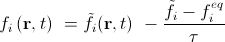
As the value of dN _coll is determined in general terms, it will remain hidden from the reader. We need only its standard approximation, Batnagar-Gross-Crook (BGK). In this approximation, dN _coll equals
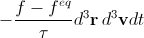$BGK approximation, - \ frac {f - f ^ {eq}} {\ tau} d ^ 3 \ mathbf {r} \, d ^ 3 \ mathbf {v} dt$ , (five)
where f ^{eq is the} equilibrium distribution function, the Maxwell-Boltzmann distribution , and τ is the so-called relaxation time .

As a result, we get
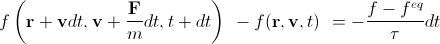$Boltzmann derivation, f \ left (\ mathbf {r} + \ mathbf {v} dt, \ mathbf {v} + \ frac {\ mathbf {F}} {m} dt, t + dt \ right) \ - f ( \ mathbf {r}, \ mathbf {v}, t) \ = - \ frac {f - f ^ {eq}} {\ tau} dt$ . (6)
Note that f ^eq depends on the macroscopic density and velocity at a given point (that is, implicitly on the coordinate and time). It is this equation that we will need in the future, but usually it is divided by dt and lead to
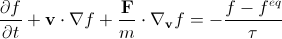$Boltzmann equation, \ frac {\ partial f} {\ partial t} + \ mathbf {v} \ cdot \ nabla f + \ frac {\ mathbf {F}} {m} \ cdot \ nabla _ {\ mathbf {v}} f = - \ frac {f- f ^ {eq}} {\ tau}$ , (7)
where nabla with index v is nabla in variable speeds.

Discrete boltzmann equation

In order to be able to model the dynamics of the continuous Boltzmann equation on a computer, we need to sample it. To do this, we first introduce a uniform grid of spatial coordinates — let the grid step be the same across all axes. The behavior of the fluid, we will determine it in the grid nodes. In fact, we only allow molecules to exist in certain spatial nodes. In addition, we must discretize time — we will determine the state of the fluid at equidistant moments of time. In addition, we will allow the molecules to have only certain values of speed — such that they have time to move to some neighboring node in a time step. These allowed directions will be the same for all spatial nodes. It is obvious that in the diagonal directions the speed of the particles will be greater than in the non-diagonal.

Intuitively, it can be concluded that with an infinitely small time step and a spatial lattice step, this discrete system transforms into the usual Boltzmann equation, which, in turn, passes to the Navier-Stokes equation in the macroscopic limit. Oddly enough, this is not such a simple question, and we will postpone it for now.

In the following exposition it is assumed everywhere that the system of units is such that the lattice spacing is a unit of length, and the time step is a unit of time.

For simplicity, below we assume that there are no external forces. We enumerate the allowed speed directions from 1 to Q with the index i. If now the mass of particles flying from a given node in the direction of i in a time step is designated as f _i , then equation (6) will go to
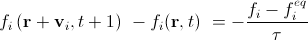$Discrete Boltzmann, f_i \ left (\ mathbf {r} + \ mathbf {v} _i, t + 1 \ right) \ - f_i (\ mathbf {r}, t) \ = - \ frac {f_i - f_i ^ {eq }} {\ tau}$ . (eight)
Here we took into account that the time step is equal to one, and replaced all dt from (6) by one. f _i ^eq denotes a discrete equilibrium distribution density, depending on the macroscopic mass and velocity at a given node. We did not specify from which node we would use f _i ^{eq —} from r + v _i t at time t + 1 or from r at time t. For the computational scheme, it is more convenient to use the node r + v _i t at the moment of time t + 1. Then the equation above can be decomposed into two components, the distribution (streaming step) and the collision (collision step).

Streaming step:
$Streaming, \ tilde {f} _i \ left (\ mathbf {r} + \ mathbf {v} _i, t + 1 \ right) \ = f_i (\ mathbf {r}, t) \,$ . (9)
Collision step:
$Collision, f_i \ left (\ mathbf {r}, t \ right) \ = \ tilde {f} _i (\ mathbf {r}, t) \ - \ frac {\ tilde {f} _i - f_i ^ {eq} } {\ tau}$ . (ten)

Here f _i with a tilde denotes the mass of particles that have come to the node in the direction i, but have not yet collided with the rest of the particles. Streaming step is sometimes called advection step.

For discrete velocity directions, the mass and macroscopic velocity at each node will be calculated as
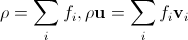$Density and velocity discrete, \ rho = \ sum_ {i} f_i, \ rho \ mathbf u = \ sum_ {i} f_i \ mathbf v_i$ . (eleven)

Hereinafter, we write density everywhere instead of mass, since with a single spatial lattice spacing there is a unit volume for each node, and the mass and density coincide in value.

We will show that the equilibrium distribution functions depend on the mass in the nodes and the macroscopic velocity. Therefore, after the streaming step, it is necessary to recalculate the masses and velocities at each node, recalculate the equilibrium distribution functions, and then perform a collision.

Thus, at each step of the computational scheme, it is necessary to “distribute” particles, that is, to move particles flying from node r in direction i to node r + v _i (do this for all particles and directions). After this, it is necessary to recalculate masses, velocities, and equilibrium distribution functions. Finally, it is necessary to “collide” particles that have flown into a given node — that is, to redistribute the particles in directions.

Illustration of computational scheme

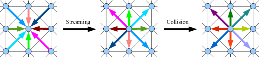
We illustrate the computational scheme on the example of a two-dimensional system. The discretization into spatial nodes and the relations between them (that is, the allowed directions of velocity) are shown in the figure below. Spatial nodes are indicated by circles, the connections between them are thin lines.
D2Q9

The following image shows one iteration of the streaming / collision pair. Colored arrows represent the flow of flying molecules. The intensity of the color encodes the mass of molecules flying in a given stream, the length of the arrows roughly corresponds to the path that the stream passes over the time step (only approximately, since the arrows must go from the center of the node to the center of the node).
CollisionAdvection

Spatial lattices

In LBM, lattice (lattice) refers to the set of allowed velocity vectors (the same for each spatial node). This is consistent with the standard mathematical definition of the lattice as an entity, with the help of which the entire spatial grid can be obtained by means of parallel translations.

In LBM, any lattice must contain a zero vector from a node to itself — it describes particles that do not fly anywhere from a given node. In LBM, lattices are usually denoted by the abbreviation DnQm, where n is the dimension of space, m is the number of vectors in the lattice. For example, D2Q9, D3Q19, etc.

In a two-dimensional LBM space, the lattice can consist, for example, of 5 vectors (2 vertical, 2 horizontal and zero vector from a node into itself), and maybe 9 vectors, as in the illustration above (2 vertical, 2 horizontal, 4 diagonal, one null). These are the D2Q5 and D2Q9 grids, respectively.

Obvious factors for the choice of gratings are: 1. modeling accuracy (intuitively, the more vectors in the grid, the more accurate the modeling) 2. computational costs (calculation on the D2Q5 grid will be faster than the calculation on D2Q9). Oddly enough, these are not the most important factors. The most important factors are the reproducibility of the Navier-Stokes equations and the symmetry of some tensors built on lattice vectors.

The gratings D2Q9, D3Q15, D3Q19 are commonly used. The grilles D2Q9 and D3Q19 are shown below. The basis vectors of the lattice are usually denoted as e _i or c _i (they coincide with the velocities v _i , introduced earlier at a single time step). Below we will use the notation e _i .

D2Q9

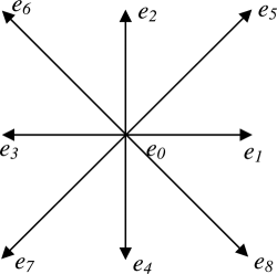
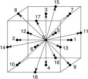
We write the basic vectors for D2Q9:
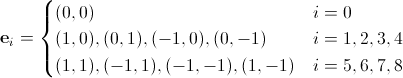$D2Q9 vectors \ bold {e} _i = \ begin {cases} (0,0) & i = 0 \\ (1,0), (0,1), (- 1,0), (0, -1) & i = 1,2,3,4 \\ (1,1), (- 1,1), (- 1, -1), (1, -1) & i = 5,6,7,8 \ \ \ end {cases}$ (eleven)

and for D3Q19:
$D3Q19 vectors \ bold {e} _i = \ begin {cases} (0,0,0) & i = 0 \\ (\ pm 1,0,0), (0, \ pm 1,0), (0, 0, \ pm 1) & i = 1,2, ..., 5,6 \\ (\ pm 1, \ pm 1,0), (\ pm 1,0, \ pm 1), (0, \ pm 1, \ pm 1) & i = 7,8, ..., 17,18 \\ \ end {cases}$ (12)

Let me remind you once again that everywhere we assume that the time step is equal to one, therefore v _i = e _i .

Equilibrium distribution functions

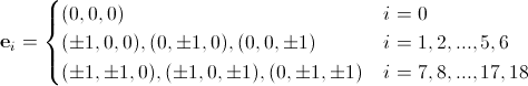
In the continuous case, the equilibrium distribution function ( Maxwell-Boltzmann distribution ) is equal to
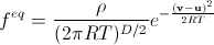$Maxwell distribution, f ^ {eq} = \ frac {\ rho} {(2 \ pi RT) ^ {D / 2}} e ^ {- \ frac {(\ bold {v} - \ bold {u}) ^ 2} {2RT}}$ . (13)

Here there are no previously encountered quantities: R is the universal gas constant , T is the temperature, D is the dimension of space, v is the velocity vector, the probability density for which we find. Here, the molar mass of the gas is taken equal to unity (it is not important for us — only macroscopic density is important). It can be considered a change in the unit of mass in our simulation. In addition, the function is normalized to local macroscopic density, and not per unit. Note also that usually the macroscopic gas velocity u is not subtracted from v. This is because the distribution is usually investigated in the case of a stationary gas, we also need to go to a local inertial reference system moving with the current gas velocity at a given point at a given time to use the Maxwell-Boltzmann distribution. Subtracting u is such a transition.

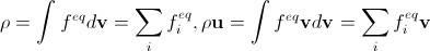
Suppose that at a given point in space, the velocity distribution of molecules turned out to be equilibrium. This distribution depends on the macroscopic mass ρ and the velocity u. On the other hand, we can calculate ρ and u from the distribution function (see formulas (2) and (3)). Obviously, this calculation should give correct ρ and u (that is, in a sense, this is an additional restriction on the distribution function):
$Density equilibrium, \ rho = \ int f ^ {eq} d \ mathbf v$ , $Velocity equilibrium, \ rho \ mathbf u = \ int f ^ {eq} \ mathbf v d \ mathbf v$ . (14)

We impose the same requirement on the density and velocity calculations in the discrete case:
$Density and velocity discrete equilibrium, \ rho = \ sum_ {i} f ^ {eq} _i, \ rho \ mathbf u = \ sum_ {i} f ^ {eq} _i \ mathbf v_i$ . (15)

The main requirement for discrete equilibrium distribution functions is the reproduction of the Navier-Stokes equation in the limit of an infinitely small time step and lattice step. This is equivalent to the fact that if, for given ρ and u, we try to calculate them again from the equilibrium distribution functions in the continuous and discrete case, the results will coincide (see the remark above that in the discrete case instead of density we mean mass), t. e.
$Density and velocity equality, \ rho = \ int f ^ {eq} d \ mathbf v = \ sum_ {i} f ^ {eq} _i, \ rho \ mathbf u = \ int f ^ {eq} \ mathbf vd \ mathbf v = \ sum_ {i} f ^ {eq} _i \ mathbf v$ . (sixteen)

In order to unambiguously determine the equilibrium discrete distribution function, we will also need to include the analogous requirement of equality of macroscopic thermal energies at a given point; we omit it for brevity.

If we sum up in the directions of the velocity equation (10) for a collision step, then, taking into account formula (16), it can be shown that the collision step does not change the macroscopic masses and velocities of the molecules in the node.

It turns out that if we simply substitute the discrete velocity vectors e _i = v _i from (11) and (12) into the continuous equilibrium distribution function (13), equalities (16) will not be fulfilled.

It also turns out that we can force equalities (16) to hold if we decompose the Maxwell-Boltzmann distribution (13) into a Taylor series to a second order macroscopic velocity. This corresponds to the fact that the value of u / sqrt (RT) is very small. This restriction must always be met during the modeling process on all nodes.

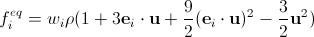
But even decomposing into a Taylor series is not enough. We must also introduce specially chosen factors w _i into the sampled functions f _i ^eq (the details of the calculations can be found in this excellent article — there is also a free version; Of course, everything will turn out to be a little more complicated than in our superficial description — in fact, the calculation takes place through tensors, up to the fourth rank, built on lattice vectors). Finally we get
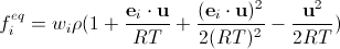$Maxwell distribution discrete, f^{eq}_i = w_i \rho (1+\frac{\vec{v_i} \cdot \vec{u}}{RT}+\frac{(\vec{v_i} \cdot \vec{u})^2}{2(RT)^2}-\frac{\vec{u}^2}{2RT})$ . (17)

Here lies the catch: we always assume that the lattice spacing and time are units of length and time, respectively. Therefore, we cannot take the value of R from SI, and the temperature here is not equal to the temperature of the simulated liquid in Kelvin.

To determine their values, note the following. Suppose there is a disturbance in the fluid — that is, there is an excess mass in some nodes. This mass will begin to “spread out” in space, moreover, in the rightmost node in the area of perturbation, it will also move in the direction (1, 0, 0) in 3D or (1, 0) in 2D. For a unit of time, molecules along these directions will pass a unit of length, that is, their speed will be equal to unity. This means that the speed of sound as the speed of propagation of disturbances in our system is also equal to one. On the other hand, the speed of sound is equal to sqrt (γ RT / μ), where γ is the adiabatic constant , μ is the molar mass, which we took equal to unity earlier. The adiabatic constant γ is 1 + 2 / d, where d is the number of degrees of freedommolecules. In ideal gas it is equal to the dimension of space. In our gas, molecules can only move along straight lines connecting nodes, therefore the dimension is not three (or two), but one. That is, γ = 3 and sqrt (3 RT) = 1.

Usually in the literature on LBM, “speed of sound” is understood as
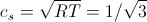$Speed of sound, c_s = \sqrt{RT}=1/\sqrt{3}$ . (18)

Now, finally,
$Maxwell distribution discrete, f^{eq}_i = w_i \rho (1+3\mathbf{e}_i \cdot \mathbf{u}+\frac{9}{2}(\mathbf{e}_i \cdot \mathbf{u})^2-\frac{3}{2}\mathbf{u}^2)$ . (nineteen)

We write the values of the coefficients w _i for the most common lattices.
For D2Q9:
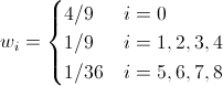$D2Q9 weights w_i = \begin{cases} 4/9 & i = 0 \\ 1/9 & i = 1,2,3,4 \\ 1/36 & i = 5,6,7,8 \\ \end{cases}$ (20)

For D3Q19:
$D3Q19 weights w_i = \begin{cases} 1/3 & i = 0 \\ 1/18 & i = 1,2,...,5,6 \\ 1/36 & i = 7,8,...,17,18 \\ \end{cases}$ (21)

Incompressibility

The limitation on the small macroscopic velocity of a fluid can now be written as
$Incompressibility, u << speed\ of\ sound = 1$ . (22)

Recall that the Mach number is the ratio of the characteristic gas velocity in the system to the speed of sound. Then the limit above corresponds to small Mach numbers or incompressible fluid. Indeed, if the speed of sound (the velocity of propagation of density perturbations) is large, then any density perturbation will quickly spread to the entire system, and the density will again become the same. That is, to compress the liquid in any one local area you will not succeed.

A good maximum value for macroscopic speed in nodes will be, for example, 0.01.

Viscosity and reynolds number

The kinematic viscosity ν in LBM (as usual in lattice units) is calculated as
$Viscosity, \nu = (\tau - 1/2)c^2_s = (\tau - 1/2)/3$ . (23)
Here τ is the relaxation time introduced earlier in formula (5), c _s = 1 / sqrt (3) is the “speed of sound” introduced in (18).

When modeling hydrodynamics exclude any system temperature changes with prescribed geometry (e.g., a pipe with a square cross-section) is completely described by only one parametrom- dimensionless Reynolds number , equal to
$Reynolds, Re = v L / \nu$ , (24)
where v-speed characteristic in the system (e.g., velocity at the center of the pipe ), L is the characteristic length in the system (for example, the length of the side of the square of the section).

For standard geometries, the relationship between characteristic velocity and external force (which provides flow) is usually known. Therefore, for modeling with a given Reynolds number,

choose characteristic speed v. As we found out, it should be much less than the speed of sound. For example, 0.01.
calculate the required external force for this speed
calculate the viscosity by (23) so as to obtain the desired Reynolds number
calculate the relaxation time by (24) so as to obtain the desired viscosity

If the modeling problem is composed in SI units (they say, the side of the square of the pipe section is 1 m, the pressure at the pipe inlet is X Pascal, and the output is Y Pascal), then you must first find the dimensionless Reynolds number and use the algorithm above.

Once again all together

Before modeling it is necessary to set the initial macroscopic masses and velocities at each node. Then specify the mass flows in each allowed direction e _i at each node (see Reefs). The easiest way is to indicate the flows from the equilibrium distribution.

To simulate in a loop commit

streaming step by the formula (9)
recalculation of macroscopic masses and speeds in each node by formulas (11), recalculation of equilibrium flows in all directions according to formula (19)
collision step by the formula (10)

Simulation usually occurs until the system is in a stationary state. Stationarity can be checked, for example, through the difference in macroscopic velocities and masses at each node between adjacent steps, the maximum among all nodes.

miscellanea

Additions to the algorithm

We have not touched upon the inclusion of external forces in modeling (for example, gravity). They will lead to a small addition to equation (9) for the streaming step.

We also did not touch the boundary conditions — on the surface of bodies and on the system inlet and outlet (for example, if a constant pressure or velocity field is specified at the pipe inlet). LBM has great freedom in modeling such conditions, since the method is formulated at the microscopic level (molecular flows), and such boundary conditions at the macroscopic level. There are many ways to set boundary conditions at the microscopic level — and many algorithms .

The boundary conditions at the boundary of solids in hydrodynamics are usually chosen as the no-slip boundary conditions (that is, when the velocity of the liquid on the surface of the bodies is zero). Usually they are realized through bounce-back conditions (when the flows of molecules are reflected in the opposite direction when crossing a solid wall). This can be read here , section 4.6.

The model of the collisions we presented is called single relaxation time. There are more advanced models, for example, multiple relaxation time (in particular, double relaxation time).

LBM also supports multiphase (simulating the flow of a mixture of liquids or gases with different parameters).

The presence of heat conduction (that is, heat transfer in the system, temperature changes at different points in the system and, as a result, changes in system parameters — for example, density) is also supported by LBM . Temperature is modeled as a separate "gas", also according to the LBM algorithm, but the velocity of this gas is determined by the velocity of the main fluid. It is said that the temperature in this sense is passive scalar. There are quite a few articles on LBM modeling of Rayleigh – Benard convection phenomena .

We didn’t touch upon the issues of efficient implementation and parallelization.

Underwater rocks

If you are modeling a system with thermal conductivity, then it will be described by two dimensionless quantities. In the case of Rayleigh-Benard convection, the Prandtl number and the Rayleigh number are usually chosen . In order to reproduce this system in lattice units, it is not enough just to reproduce both of these dimensionless quantities, by correctly setting the internal parameters of the system (characteristic speed, external force, thermal conductivity). The fact is that between the internal parameters there will be hidden dependencies. You can read more here .

As we have already said, when choosing the characteristic speed in the system, do not forget that the Mach number must be much less than one (formula (22)).

LBM can become unstable in some systems at high Reynolds numbers (when the flow, however, is still laminar). Galilean invariance is not satisfied

in LBM . However, it usually does not matter. At the beginning of the simulation, it is necessary to specify the flows of molecules from each node in all allowed directions. Often choose the equilibrium distribution of flows (formula (19)). It is important to remember that equilibrium does not imply stationarity. That is, stationary distributions in the presence of velocity gradients, external forces, etc. differ from equilibrium. Their calculation is given here (formulas 12, 19, 20 by reference).

Existing solutions

There is a large and very mature open-source project entirely dedicated to LBM — Palabos (PA Parallel LAttice BOLtzmann). The project has a wiki . Developers provide paid advice on hydrodynamic modeling.

There are excellent teaching examples of modeling typical MATLAB systems. For example, Rayleigh – Benard convection (external force is available, thermal conductivity, boundary conditions, correct translation of quantities). Only 160 lines in MATLAB.

There are many commercial solutions, for example, this or that .

A detailed list of commercial and non-commercial packages can be found on Wikipedia .

What to read

In addition, you can recommend these lists of articles and books . Basically a list of books is on Wikipedia .

That's all,

Thanks for attention!

Source: https://habr.com/ru/post/190552/

All Articles