Neural network in practice: The task of a traveling salesman
Good afternoon, dear habro users.
I would like to share the practical application of one of the neurodynamic algorithms, in the continuation of my post. Modeling the neural network of the Boltzmann Machine .
Implementation on the example of solving the traveling salesman problem.
I will remind a little of what its essence is.

The task of the traveling salesman (traveling salesman (Fr. commis voyageur, outdated) - traveling sales broker) is to find the most profitable route passing through the specified cities. In terms of the task, the criterion of the route profitability (shortest, cheapest, aggregate criterion, etc.) and the corresponding matrices of distances, costs, etc. are indicated. As a rule, it is indicated that the route should pass through each city only once - in such case, the choice is carried out among Hamiltonian cycles.
To solve this problem, a network consisting of 100 neurons is used.
When assigning weights, there must be a guarantee that the neural network provides a solution that matches the correct tour. It becomes clear why the assignment of weights is most significant for achieving a good solution when using the Boltzmann machine and the Hopfield network. Hopfield and Tank suggested one way to assign weights to the Boltzmann machines. The main idea is to impose fines on incorrect tours and at the same time minimize the length of the tour. The Aarts approach makes it possible to formally establish assignments by associating with the task, while many other approaches for assigning weights are heuristic. Of course, it does not necessarily mean that the resulting algorithm works well, so Aarts offers several modifications designed to improve the performance of large tasks.
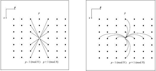
Fig.14 Fig. 15
Figures (14) and (15) illustrate the connections made to each network node. They are divided into two types. Connections of distances for which the weights are chosen in such a way that if the network is in a state that corresponds to the tour, these weights will reflect the energy cost of the connection (p-1) of the tour city with p city, and p - the city with the city (p + 1).
The figure (14) shows the distance connections. Each node (i, p) has prohibiting links to two adjacent columns, whose weights reflect the cost of connecting the three cities.
Figure (15) shows the exclusive connections. Each node (i, p) has prohibiting links to all elements in the same row and column.
')
Exclusive connections prohibit two elements from being in the same row or column at the same time. Exclusive connections allow the network to be set to the state of the corresponding tour.
Since all connections are so far prohibiting, we need to provide the network with some incentive to include elements, by manipulating thresholds. Intuitively, we can see that some arrangements, such as those shown in figures (14) and (15), may have the desired effect, but the following theorem shows how to accurately select weights. Consider the following set of parameters:
")
)")
 \ cap (i \ neq j \ cup p = q))")
(13)
Where, dij is the distance between i and j cities, N is the number of cities, eipjq is the energy between neurons (j, q) and (i, p).
Note that each element in Figures (14) and (15) is in the table, therefore any particular element is identified by two signatures. θip is the input of the element (i, p), and wipjq is the weight from the element (j, q) to (i, p).
Select weights and inputs so that
")

")
(14)
Then
1. Feasibility. Correct states of network tours correspond exactly to the local minimum of energy
2. Streamlining. The energy function is order saving according to the length of the tour.
The proof is fairly straightforward and depends on the demonstration that the states of the tours correspond exactly with the local minimum of energy. In a Boltzmann asynchronous machine, the local energy minima correspond exactly with fixed points. The disadvantage of the algorithm is that in the synchronous case, some local minima of energy can also correspond to two cycles, which complicates the assignment of weights in the synchronous case.
When solving the traveling salesman problem, the functioning of the network is as follows:
1. Calculated scales, taking into account the task, according to the algorithm described above.
2. Input signal
3. The neurons are activated according to the Boltzmann learning algorithm, except that the weights remain always the same.
4. Repeat steps 2 and 3 until the energy reaches the global minimum (i.e., during n calculations, does not change its state).
Optimization of the algorithm
Solving the problem with the help of the “Annealing Simulation” algorithm, in addition to the correct selection of weights, the input vector, threshold values and dimensions, the parameter t (temperature) is equally important.
The metal is annealed, heating it to a temperature above its melting point, and then letting it cool down slowly. At high temperatures, atoms, having high energies and freedom of movement, randomly accept all possible configurations. With a gradual decrease in temperature, the energy of atoms decreases, and the system as a whole tends to adopt a configuration with minimal energy. When cooling is complete, a global minimum energy state is reached.
At a fixed temperature, the energy distribution of the system is determined by the Boltzmann probability factor.
Hence it is obvious: there is a finite probability that the system has high energy even at low temperatures. In a similar way, there is a small but calculated probability that a kettle with water on fire will freeze before it boils.
The statistical distribution of energy allows the system to exit from local minima of energy. At the same time, the probability of high-energy states decreases rapidly with decreasing temperature. Therefore, at low temperatures, there is a strong tendency to occupy a low-energy state.
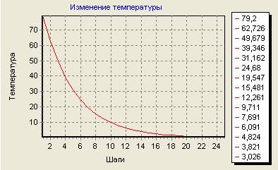
For a more flexible temperature change, the entire graph was divided into intervals in which the user can change the temperature drop rate himself (up to 50 iterations, from 50 to 120 iterations, more than 120 iterations).
In the process of practical research the following patterns were derived:
1. At high temperatures, the energy behaves erratically, when at low temperatures it becomes almost deterministic.
2. Changing the temperature to any constant in any interval, most often the algorithm finds a path between all cities, but at most it is far from optimal.
3. To obtain the most accurate answer, it is necessary at low temperatures to significantly reduce the rate of fall of the parameter t, which is not the case for high temperatures. When the temperature is maximum, the speed of the fall has almost no effect on the result.
In the course of these studies, we found that temperature is much more important than any other parameter involved in the calculations, in order to achieve the most accurate result (in this case, the shortest path between cities). This can be achieved by reducing the rate of decline of the parameter t in the final part of the calculations. In the network model we use, it is recommended to perform a decrease in the interval “after 120 iterations”.
For a visual representation of the results obtained in the network modeling program developed by us, we present a graph of the temperature at which the optimum result was achieved.
Studies have also been made in the area of neural network activation. In addition to the standard change of state in each individual neuron, selected at random, activation is performed by a group of neurons (in this model, the group includes 10 neurons). Each neuron in this group changes its state to the opposite. This method of activation allows you to even more parallelize the computation process, which leads to a more rapid finding of the right solution. The number of calculation steps was reduced from 534 to 328.
Thus, it is possible to optimize this neural network not only with respect to accuracy, changing the temperature graph, but also the speed of finding the right answer, by increasing the number of neurons that change their state at one time.
I would like to share the practical application of one of the neurodynamic algorithms, in the continuation of my post. Modeling the neural network of the Boltzmann Machine .
Implementation on the example of solving the traveling salesman problem.
I will remind a little of what its essence is.
The task of the traveling salesman (traveling salesman (Fr. commis voyageur, outdated) - traveling sales broker) is to find the most profitable route passing through the specified cities. In terms of the task, the criterion of the route profitability (shortest, cheapest, aggregate criterion, etc.) and the corresponding matrices of distances, costs, etc. are indicated. As a rule, it is indicated that the route should pass through each city only once - in such case, the choice is carried out among Hamiltonian cycles.
To solve this problem, a network consisting of 100 neurons is used.
When assigning weights, there must be a guarantee that the neural network provides a solution that matches the correct tour. It becomes clear why the assignment of weights is most significant for achieving a good solution when using the Boltzmann machine and the Hopfield network. Hopfield and Tank suggested one way to assign weights to the Boltzmann machines. The main idea is to impose fines on incorrect tours and at the same time minimize the length of the tour. The Aarts approach makes it possible to formally establish assignments by associating with the task, while many other approaches for assigning weights are heuristic. Of course, it does not necessarily mean that the resulting algorithm works well, so Aarts offers several modifications designed to improve the performance of large tasks.
Fig.14 Fig. 15
Figures (14) and (15) illustrate the connections made to each network node. They are divided into two types. Connections of distances for which the weights are chosen in such a way that if the network is in a state that corresponds to the tour, these weights will reflect the energy cost of the connection (p-1) of the tour city with p city, and p - the city with the city (p + 1).
The figure (14) shows the distance connections. Each node (i, p) has prohibiting links to two adjacent columns, whose weights reflect the cost of connecting the three cities.
Figure (15) shows the exclusive connections. Each node (i, p) has prohibiting links to all elements in the same row and column.
')
Exclusive connections prohibit two elements from being in the same row or column at the same time. Exclusive connections allow the network to be set to the state of the corresponding tour.
Since all connections are so far prohibiting, we need to provide the network with some incentive to include elements, by manipulating thresholds. Intuitively, we can see that some arrangements, such as those shown in figures (14) and (15), may have the desired effect, but the following theorem shows how to accurately select weights. Consider the following set of parameters:
(13)
Where, dij is the distance between i and j cities, N is the number of cities, eipjq is the energy between neurons (j, q) and (i, p).
Note that each element in Figures (14) and (15) is in the table, therefore any particular element is identified by two signatures. θip is the input of the element (i, p), and wipjq is the weight from the element (j, q) to (i, p).
Select weights and inputs so that
(14)
Then
1. Feasibility. Correct states of network tours correspond exactly to the local minimum of energy
2. Streamlining. The energy function is order saving according to the length of the tour.
The proof is fairly straightforward and depends on the demonstration that the states of the tours correspond exactly with the local minimum of energy. In a Boltzmann asynchronous machine, the local energy minima correspond exactly with fixed points. The disadvantage of the algorithm is that in the synchronous case, some local minima of energy can also correspond to two cycles, which complicates the assignment of weights in the synchronous case.
When solving the traveling salesman problem, the functioning of the network is as follows:
1. Calculated scales, taking into account the task, according to the algorithm described above.
2. Input signal
3. The neurons are activated according to the Boltzmann learning algorithm, except that the weights remain always the same.
4. Repeat steps 2 and 3 until the energy reaches the global minimum (i.e., during n calculations, does not change its state).
Optimization of the algorithm
Solving the problem with the help of the “Annealing Simulation” algorithm, in addition to the correct selection of weights, the input vector, threshold values and dimensions, the parameter t (temperature) is equally important.
The metal is annealed, heating it to a temperature above its melting point, and then letting it cool down slowly. At high temperatures, atoms, having high energies and freedom of movement, randomly accept all possible configurations. With a gradual decrease in temperature, the energy of atoms decreases, and the system as a whole tends to adopt a configuration with minimal energy. When cooling is complete, a global minimum energy state is reached.
At a fixed temperature, the energy distribution of the system is determined by the Boltzmann probability factor.
Hence it is obvious: there is a finite probability that the system has high energy even at low temperatures. In a similar way, there is a small but calculated probability that a kettle with water on fire will freeze before it boils.
The statistical distribution of energy allows the system to exit from local minima of energy. At the same time, the probability of high-energy states decreases rapidly with decreasing temperature. Therefore, at low temperatures, there is a strong tendency to occupy a low-energy state.
For a more flexible temperature change, the entire graph was divided into intervals in which the user can change the temperature drop rate himself (up to 50 iterations, from 50 to 120 iterations, more than 120 iterations).
In the process of practical research the following patterns were derived:
1. At high temperatures, the energy behaves erratically, when at low temperatures it becomes almost deterministic.
2. Changing the temperature to any constant in any interval, most often the algorithm finds a path between all cities, but at most it is far from optimal.
3. To obtain the most accurate answer, it is necessary at low temperatures to significantly reduce the rate of fall of the parameter t, which is not the case for high temperatures. When the temperature is maximum, the speed of the fall has almost no effect on the result.
In the course of these studies, we found that temperature is much more important than any other parameter involved in the calculations, in order to achieve the most accurate result (in this case, the shortest path between cities). This can be achieved by reducing the rate of decline of the parameter t in the final part of the calculations. In the network model we use, it is recommended to perform a decrease in the interval “after 120 iterations”.
For a visual representation of the results obtained in the network modeling program developed by us, we present a graph of the temperature at which the optimum result was achieved.
Studies have also been made in the area of neural network activation. In addition to the standard change of state in each individual neuron, selected at random, activation is performed by a group of neurons (in this model, the group includes 10 neurons). Each neuron in this group changes its state to the opposite. This method of activation allows you to even more parallelize the computation process, which leads to a more rapid finding of the right solution. The number of calculation steps was reduced from 534 to 328.
Thus, it is possible to optimize this neural network not only with respect to accuracy, changing the temperature graph, but also the speed of finding the right answer, by increasing the number of neurons that change their state at one time.
Source: https://habr.com/ru/post/188938/
All Articles