Solving the problem of clustering using gradient descent
 Hey. In this article, we will discuss the method of data clustering using the gradient descent method . To be honest, this method is more academic than practical. I needed to implement this method for demonstration purposes for a machine learning course to show how identical tasks can be solved in various ways. Although of course, if you plan to cluster data using a differentiated metric, for which it is computationally more difficult to find a centroid , rather than counting a gradient on some data set, then this method may be useful. So, if you're wondering how to solve the k-means clustering problem with a generalized metric using the gradient descent method, I ask for cat. Code in R.
Data
First, let's discuss the set of data on which we will test the algorithms. For testing uses a lot of data from the sensors of smartphones : only 563 fields in 7352 observations; from the bottom 2 fields are allocated for the user ID and type of action. The set is created to classify user actions depending on sensor readings, a total of 6 actions (WALKING, WALKING_UPSTAIRS, WALKING_DOWNSTAIRS, SITTING, STANDING, LAYING). A more detailed description of the set can be found at the above link.
As you understand it, to visualize such a multitude without reducing the dimensionality is a bit problematic. To reduce the dimension, the principal component method was used; for this, you can use the standard means of the R language, or implement this method in the same language from my repository . Let's take a look at what the original set looks like, projected onto the first and third main components.
Code
m.proj <- ProjectData(m.raw, e$eigenVectors[, c(1, 3)]) plot(m.proj[, 1], m.proj[, 2], pch=19, col=rainbow(6)[unclass(as.factor(samsungData$activity))], xlab="first", ylab="third", main="Two components; actions") ')
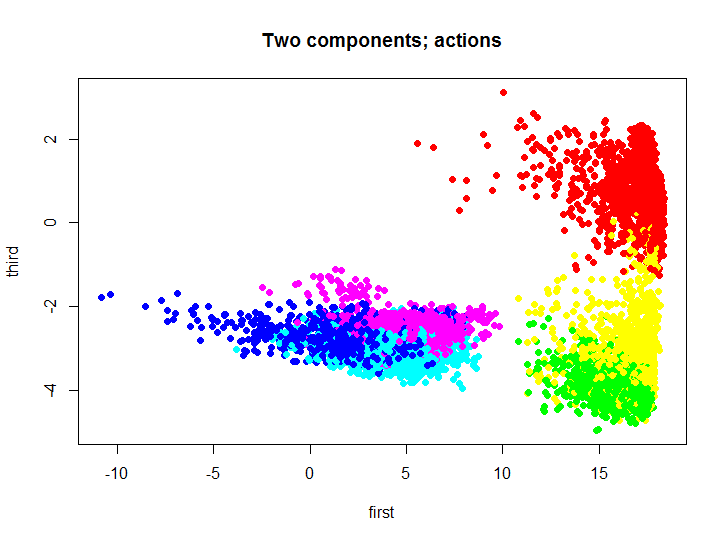
Different colors indicate different actions, then we will use this two-dimensional set to test and visualize the results of clustering.
K-means algorithm cost function
We introduce the following notation:
 - many centroids
  corresponding clusters
 - the original set of data that must be clustered
 - k-th cluster, a subset of the original set
Now consider the cost function of the classic k-means algorithm :
those. the algorithm minimizes the total square deviation of cluster elements from the centroid. In other words, the sum of squares of the Euclidean distance of cluster elements from the corresponding centroid is minimized:
 where f is in this case the Euclidean distance.
As it is known, there is an effective learning algorithm based on the expectation-maximization algorithm for solving this problem. Let's take a look at the result of this algorithm, using the built-in function in R:
Code
kmeans.inner <- kmeans(m.proj, 3) plot(m.proj[, 1], m.proj[, 2], pch=19, col=rainbow(3)[unclass(as.factor(kmeans.inner$cluster))], xlab="first", ylab="third", main=paste(k, " clusters; kmeans \n cost = ", kmeans.inner$tot.withinss/2, sep="")) 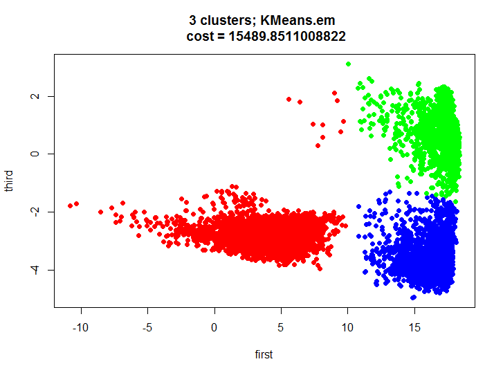
Gradient descent
The gradient descent algorithm itself is pretty simple, the point is to move in small steps towards the opposite direction of the gradient, for example, the back propagation error algorithm , or the contrastive divergence algorithm for learning the limited Boltzmann machine , works. First of all, it is necessary to calculate the gradient of the objective function, or the partial derivatives of the objective function from the model parameters.
 since we left the section on classic k-means, then f can in principle be any measure of distance, not necessarily the Euclidean metric
But there is a problem, we do not know at this stage what the partition of the set X into clusters is. Let's try to reformulate the objective function in such a way that we write it in the form of one formula that would be easy to differentiate: the sum of the minimum distances from each element of the set to one of the three centroids. This formula is as follows:
Now let's find the derivative of the new objective function:
Well, it remains to find out what the derivative of the minimum is equal to, but everything turns out to be simple: if the a- th centroid is really the one to which the distance is minimal from the current element of the set, then the derivative of the expression is equal to the derivative of the square of the distance along the vector element, otherwise case is zero:

Method implementation
As you understand, all the steps from the previous paragraph can be performed without squaring the distance. This was done in the implementation of this method. The method receives as parameters the distance function and the function of calculating the partial derivative of the distance function between two vectors by the component of the second vector, for example, “half the square Euclidean distance” (convenient to use because the derivative is very simple), as well as the function of the gradient descent :
Distance functions
Distance function
Partial derivative function
HalfSqEuclidian.distance <- function(u, v) { # Half of Squeared of Euclidian distance between two vectors # # Args: # u: first vector # v: second vector # # Returns: # value of distance return(sum((uv)*(uv))/2) } Partial derivative function
HalfSqEuclidian.derivative <- function(u, v, i) { # Partial derivative of Half of Squeared of Euclidian distance # between two vectors # # Args: # u: first vector # v: second vector # i: index of part of second vector # # Returns: # value of derivative of the distance return(v[i] - u[i]) } Gradient descent method
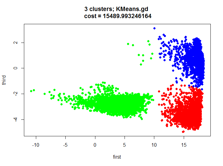
KMeans.gd <- function(k, data, distance, derivative, accuracy = 0.1, maxIterations = 1000, learningRate = 1, initialCentroids = NULL, showLog = F) { # Gradient descent version of kmeans clustering algorithm # # Args: # k: number of clusters # data: data frame or matrix (rows are observations) # distance: cost function / metrics # centroid: centroid function of data # accuracy: accuracy of calculation # learningRate: learning rate # initialCentroids: initizalization of centroids # showLog: show log n <- dim(data)[2] c <- initialCentroids InitNewCentroid <- function(m) { c <- data[sample(1:dim(data)[1], m), ] } if(is.null(initialCentroids)) { c <- InitNewCentroid(k) } costVec <- vector() cost <- NA d <- NA lastCost <- Inf for(iter in 1:maxIterations) { g <- matrix(rep(NA, n*k), nrow=k, ncol=n) #calculate distances between centroids and data d <- matrix(rep(NA, k*dim(data)[1]), nrow=k, ncol=dim(data)[1]) for(i in 1:k) { d[i, ] <- apply(data, 1, FUN = function(v) {distance(v, c[i, ])}) } #calculate cost cost <- 0 for(i in 1:dim(data)[1]) { cost <- cost + min(d[, i]) } if(showLog) { print(paste("Iter: ", iter,"; Cost = ", cost, sep="")) } costVec <- append(costVec, cost) #stop conditions if(abs(lastCost - cost) < accuracy) { break } lastCost <- cost #calculate gradients for(a in 1:k) { for(b in 1:n) { g[a, b] <- 0 for(i in 1:dim(data)[1]) { if(min(d[, i]) == d[a, i]) { g[a, b] <- g[a, b] + derivative(data[i, ], c[a, ], b) } } } } #update centroids for(a in 1:k) { for(b in 1:n) { c[a, b] <- c[a, b] - learningRate*g[a, b]/dim(data)[1] } } } labels <- rep(NA, dim(data)[1]) for(i in 1:dim(data)[1]) { labels[i] <- which(d[, i] == min(d[, i])) } return(list( labels = labels, cost = costVec )) } Testing
KMeans.gd.result <- KMeans.gd(k, m.proj, HalfSqEuclidian.distance, HalfSqEuclidian.derivative, showLog = T) plot(m.proj[, 1], m.proj[, 2], pch=19, col=rainbow(k)[unclass(as.factor(KMeans.gd.result$labels))], xlab="first", ylab="third", main=paste(k, " clusters; KMeans.gd \n cost = ", KMeans.gd.result$cost[length(KMeans.gd.result$cost)], sep="")) Let's take a look at the result of clustering and make sure that it is almost identical.
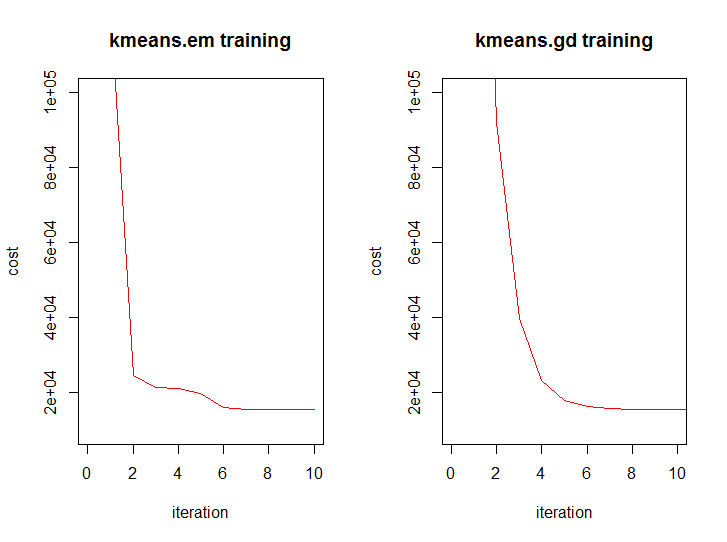
And this is how the dynamics of the value function from iteration of both algorithms look like:
Conclusion
Let's first say a few words about what happened in our test. We got a decent split of the two-dimensional set into three clusters, we visually see that the clusters do not overlap much and we can completely build models for recognizing actions for each cluster, thus we get some hybrid model (one cluster contains basically one action, the other two, and the third three).
Take a look at the complexity of the algorithms for clustering using the Euclidean distance, consider only one iteration (analyzing the number of iterations is not a trivial task at all). Let k be the number of clusters, n is the dimension of the data, m is the amount of data (k <= m). In the extreme case, k = m.
- EM version:

- GD version:

In general, mathematically, both algorithms are on the same level, but we know that one is slightly higher.
You can find all the code here .
Source: https://habr.com/ru/post/188638/
All Articles