Hidden Markov chains, Bauma-Welch algorithm
Hidden models / Markov chains are one of the approaches to data presentation. I really liked how many of these approaches are summarized in this article .
In continuation of my previous article, the description of hidden Markov models, let us ask ourselves a question: where can we get a good model? The answer is quite standard, take a good model and make it a good one.
Let me remind an example: we need to implement a lie detector, which, by trembling of human hands, determines whether it speaks the truth or not. Suppose when a person lies, his hands are shaking a little more, but we do not know how much. Take a model at random, run the Viterbi algorithm from the previous article and get some rather strange results:
There is no point in the resulting splitting; rather, there is, but not the one that I would like to see. The first question is how to estimate the likelihood of an available sample in the selected model. And the second question is how to find such a model in which the available sample would be the most plausible, that is, how to evaluate the quality and how to organize the adaptability to the new data. The forward-backward procedure and the Baum-Welch reestimation procedure are exactly what they answer.
')
The forward-backward procedure allows you to estimate the likelihood that a sample of observed values will appear in this HMM model (Designations are taken from the previous article). Denote the estimated function as
  . And we introduce two additional functions:
Functions ,
,  have the following interesting properties:

So, we can already estimate the appearance of the O sample in the HMM model and find the sequence of hidden states . It remains an open question how to find a model in which the probability of the appearance of an existing sample will be maximum, that is,
  where
where  some set of valid models. As stated, there is no formal algorithm for finding the optimum, but often you can at least a little closer to “perfection”, due to some modification of the model. This is exactly how iterative EM algorithms work .
So let's have an initial model. need to find such a model
  , what
  . Let's get started
We introduce two more auxiliary functions:
 interpreted as the fraction of transitions from state s to state s' at time t, and
  - as the total share of transitions from the state s at the moment of time t.
Modified model parameters will have the following form:
Reconfigure (NormalReestimation in our case) depends on the specific situation. The classical implementation of the algorithm assumes that the observations are described by finite discrete distributions, which does not suit us. It is proposed to use the following method for estimating parameters for observed values:
Consider the problem of a lie detector in a more general version. We have a general model of how our lie detector reacts to the lies and sincerity of the subjects and there is a specific individual who sometimes lies sometimes telling the truth. We want to customize our model to work with this, a specific individual.
Given:
It is necessary:
Decision:
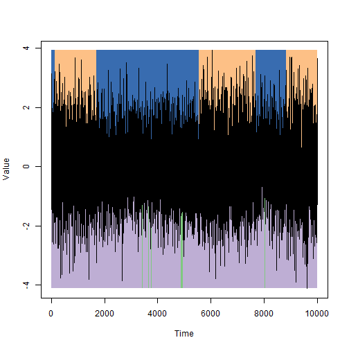
We will illustrate the answer on the data from the first picture: on top of the state, as they were set in the simulation, on the bottom, which were selected using the Markov hidden chains method.

On the graph below, we give the logarithm of the estimated function depending on the number of iterations of the Baum-Welch algorithm. The green mark is the score corresponding to the simulation parameters.

The error in estimating hidden states is relatively small, but only when the initial approximation is not much different from what we want to find. It is necessary to understand that the Baum-Welsh algorithm is just a step in the search for a local optimum, which means it may never reach a global extremum.
Formulas are converted into pictures using mathurl.com . I hope someday, here it will be possible to insert formulas in a more simple and pleasing way and, by the way, there is a lack of syntax highlighting for R.
In continuation of my previous article, the description of hidden Markov models, let us ask ourselves a question: where can we get a good model? The answer is quite standard, take a good model and make it a good one.
Let me remind an example: we need to implement a lie detector, which, by trembling of human hands, determines whether it speaks the truth or not. Suppose when a person lies, his hands are shaking a little more, but we do not know how much. Take a model at random, run the Viterbi algorithm from the previous article and get some rather strange results:
There is no point in the resulting splitting; rather, there is, but not the one that I would like to see. The first question is how to estimate the likelihood of an available sample in the selected model. And the second question is how to find such a model in which the available sample would be the most plausible, that is, how to evaluate the quality and how to organize the adaptability to the new data. The forward-backward procedure and the Baum-Welch reestimation procedure are exactly what they answer.
')
The forward-backward procedure allows you to estimate the likelihood that a sample of observed values will appear in this HMM model
(Designations are taken from the previous article). Denote the estimated function as . And we introduce two additional functions:AlphaFunc<-function(S,I,T,P,O,Tm) { la<-I*Es(P,O[1]) alpha<-cbind(la) for(t in 2:Tm) { la<-as.vector((la*Es(P,O[t]))%*%T) alpha<-cbind(alpha,la) } return (alpha) } BetaFunc<-function(S,I,T,P,O,Tm) { lb<-rep(1,length(S)) beta<-cbind(lb) for(t in Tm:2) { lb<-as.vector(T%*%(Es(P,O[t])*lb)) beta<-cbind(lb, beta) } return (beta) } Functions
, have the following interesting properties:So, we can already estimate the appearance of the O sample in the HMM model and find the sequence of hidden states
. It remains an open question how to find a model in which the probability of the appearance of an existing sample will be maximum, that is, where some set of valid models. As stated, there is no formal algorithm for finding the optimum, but often you can at least a little closer to “perfection”, due to some modification of the model. This is exactly how iterative EM algorithms work .So let's have an initial model.
need to find such a model , what . Let's get startedWe introduce two more auxiliary functions:
xiGamma<-function(t,alpha,beta,S,T,P,O) { xi<-matrix(0,nrow=length(S),ncol=length(S)) denom<-alpha[,t]%*%beta[,t] for(sin in S) { for(sout in S) { nom<-alpha[sin,t]*T[sin,sout]*Es(P,O[t+1])[sout]*beta[sout,t+1] xi[sin,sout]<-nom/denom } } return(list(xi=xi,g=rowSums(xi))) } XiGammas<-function(Tm,alpha,beta,S,T,P,O) { xis<-c() gs<-c() for(t in 1:(Tm-1)) { xg<-xiGamma(t,alpha,beta,S,T,P,O) xis<-cbind(xis,as.vector(xg$xi)) gs<-cbind(gs,as.vector(xg$g)) } return(list(xi=xis,g=gs)) } interpreted as the fraction of transitions from state s to state s' at time t, and - as the total share of transitions from the state s at the moment of time t.Modified model parameters
will have the following form: BaumWelshFunc<-function(S,I,T,P,O,Tm) { a<-alphaLog(S,I,T,P,O,Tm) b<-betaLog(S,I,T,P,O,Tm) xg<-XiGammas(Tm, a,b, S,T,P,O) xi<-rowSums(xg$xi) dim(xi)<-c(length(S),length(S)) g<-rowSums(xi) new_I <- g/sum(g) small_t<-rep(g,length(S)) dim(small_t)<-c(length(S),length(S)) new_T <- xi/small_t norm_params<-NormalReestimation(xg$g,O[1:(Tm-1)],S) new_P<-c() for(s in S) { new_P<-c(new_P,Curry("dnorm",mean=norm_params$mu[s], sd=sqrt(norm_params$sigma2[s]))) } return(list(S=S,I=new_I,T=new_T,P=new_P,N=norm_params)) } Reconfigure
(NormalReestimation in our case) depends on the specific situation. The classical implementation of the algorithm assumes that the observations are described by finite discrete distributions, which does not suit us. It is proposed to use the following method for estimating parameters for observed values: NormalReestimation<-function(g,O,S) { denom<-rowSums(g) mu<-g%*%O/denom sigma2<-c() for(s in S) { s2<-g[s,]%*%(O-mu[s])^2 sigma2<-c(sigma2,s2) } return(list(mu=as.vector(mu),sigma2=sigma2/denom)) } Consider the problem of a lie detector in a more general version. We have a general model of how our lie detector reacts to the lies and sincerity of the subjects and there is a specific individual who sometimes lies sometimes telling the truth. We want to customize our model to work with this, a specific individual.
Given:
- Model. There are two hidden states when a spherical person is telling the truth and when lying. In either case, the twitching of the arms can be thought of as white noise, but the dispersion
- A sample of 10,000 consecutive observations of our individual.
It is necessary:
- Estimate the variance of shaking hands in the case of sincerity / falsehood of this individual.
- Determine the moments of the change of these states for him.
Decision:
- Let's set our top five:
- Number of states
 ;
; - States
 ;
; - Initial distribution
 ;
; - By default, we assume that the states are equal and, say, a change occurs on average, every 999 ticks of time:
 ;
;  where
where  .
.
I will explain that - this is the sample variance for the entire sample. Initial evaluation functions for
  are chosen in such a way that the first state corresponds to smaller values of the variance, and the second one to larger ones. Essentially, they are different.
- Number of states
- We will reconfigure the parameters using the Baum-Welsh algorithm until the value of the evaluation function stabilizes.
- We find the most plausible hidden states for each point in time using the Viterbi algorithm.
We will illustrate the answer on the data from the first picture: on top of the state, as they were set in the simulation, on the bottom, which were selected using the Markov hidden chains method.
On the graph below, we give the logarithm of the estimated function depending on the number of iterations of the Baum-Welch algorithm. The green mark is the score corresponding to the simulation parameters.
The error in estimating hidden states is relatively small, but only when the initial approximation is not much different from what we want to find. It is necessary to understand that the Baum-Welsh algorithm is just a step in the search for a local optimum, which means it may never reach a global extremum.
Formulas are converted into pictures using mathurl.com . I hope someday, here it will be possible to insert formulas in a more simple and pleasing way and, by the way, there is a lack of syntax highlighting for R.
Source: https://habr.com/ru/post/188244/
All Articles