SOINN - self-learning algorithm for robots
Post number 1. What is SOINN
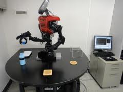
SOINN is a self-organizing incremental neural network. The structure and algorithm of such a neural network seems to have worked well in the Japanese laboratory Hasegawa (site - haselab.info ), because it was eventually taken as a basis and the further development of algorithms of artificial intelligence went through small modifications and add-ins to the SOINN network.
The core network SOINN consists of two layers. The network receives the input vector and on the first layer after training creates a node (neuron) - the defining class for the input data. If the input vector is similar to the existing class (the measure of similarity is determined by the learning algorithm settings), then the two most similar neurons of the first layer are connected by a link, or if the input vector is not similar to one existing class, then the first layer creates a new neuron that defines the current class. Very similar neurons of the first layer, combined by a link, are defined as one class. The first layer is the input layer for the second layer, and according to a similar algorithm, with a few exceptions, classes are created in the second layer.
')
On the basis of SOINN such networks are created as (the network name and the description of the network from its creators are presented below):
ESOINN - expansion of the SOINN neural network is trained online without third-party intervention and without setting a learning task. This is an improved version of the SOINN network for on-line uncontrolled classification and training topology. 1 - this network consists of one layer as opposed to two layers in SOINN; 2 - its clusters with high density of overlap; 3 - it uses fewer parameters than SOINN; and 4 - it is more stable than SOINN. Experiments on demo data and real data also show that ESOINN works better than SOINN.
ASC data classifier based on SOINN. It automatically determines the number of prototypes and assimilates new information without deleting the information already stored. It is resistant to noisy data, the classification is very fast. In the experiment, we use both demo data and real data sets to illustrate ASC. In addition, we compare ASC with other results based on classifiers, taking into account its classification of errors, compression and speed of classification. The results show that ASC has better performance and is a very effective classifier ( Reference to the original ).
GAM - General Associative Memory (GAM) is a system that combines the functions of another type of associative memory (AM). GAM is a network consisting of three layers: an input layer, a memory layer, and an associative layer. The input layer accepts input vectors. A memory layer saves input to similar classes. The associative layer builds associative connections between classes. GAM can store and call binary or non-binary information, build many-to-many associations, store and recall both static data and a temporary sequence of information. May recall information even if it has incomplete input data or noisy data. Experiments using real-time binary data using static data and time sequence data show that GAM is an efficient system. In experiments using human-like robots, it demonstrates that GAM can solve real problems and build connections between data structures with different sizes ( Reference to the original ).
The new STAR-SOINN (STAtistical Recognition - Self-Organizing and Incremental Neural Networks) - to build a smart robot, we must develop the psychic system of an autonomous robot that consistently and quickly learns from man, his environment and the Internet. Therefore, we offer the STAR-SOINN network - this is an ultra-fast, multi-modal network that learns in real time and has the ability to additionally learn via the Internet. We conducted experiments to evaluate this teaching method and compared the results with other teaching methods. The result shows that recognition accuracy is higher than a system that simply adds conditions. In addition, the proposed method can work very quickly (for about 1 second to study an object, 25 milliseconds, for object recognition). The algorithm was able to identify the attributes of "unknown" objects by searching for the attribute information of known objects. Finally, we decided that this system potentially becomes the base technology for future robots.
SOIAM - modification SOINN for associative memory.
SOINN-PBR - modification of SOINN to create rules using conditions if -> then (if-then)
AMD (Autonomous Mental Development) - a robot using this algorithm to learn to solve various problems.
The block diagram of the SOINN algorithm can be found here.
A link to the magazine in pdf format, where a description of several SOINN networks in English is given and where I made notes in Russian (I packed the rar archive, the original magazine size was 20 mb ( read online ), the archive size was 13 mb ( download archive ).
Link to another magazine in pdf format, which describes several varieties of SOINN networks in English and where I made notes in Russian (I packed the rar archive, the original journal size was 4mb ( read online ), the archive size was 2.5mb ( download archive ).
In the Russian-language Internet about the SOINN network, there are only a couple of articles that the robot, working according to this algorithm, finds solutions to the problems and if it is not explained how to solve the problem, then it connects to the Internet and looks for a solution there. But I did not find examples of the operation of the algorithm and codes. Only there was one article on robocraft where a small example of the operation of the basic algorithm of the SOINN network in conjunction with OpenCV is given. If someone experimented with the SOINN network, it would be interesting to look at the code, if possible.
Back in 2006, a method of gradual (increasing) learning was proposed, called the self-organizing growing neural network (SOINN), in order to try to implement unsupervised learning (self-study without a teacher). SOINN does a good job of processing non-stationary data online, reports the number of defined clusters, and represents the topological structure of the input data, taking into account the probability of the probability distribution density. Hasagawa, who proposed a version of the SOINN network, compared the results of his network operation with the GNG network (expanding neural gas) and the result of the SOINN network was better than that of the GNG network.
There were such problems with the SOINN network:
1. Due to the fact that it consisted of two processing layers, that the user had to take part in the network. The user had to decide when to stop learning the first layer and when to start acquiring knowledge in the second layer.
2. If the groups have high density, then the network coped well with their recognition, but if the network of the group partially overlapped, then the network thought it was one group and united them.
To solve these problems and simplify the network architecture, a SOINN-based network with increased self-organization was proposed and called ESOINN.
SOINN Short Review.
Soinn consists of a network with two layers. The first layer studies the distribution density of the input data and uses the nodes and the connections between them to represent the result of the data distribution. The second layer searches for data in the first layer with the lowest distribution density and identifies groups for them and uses fewer nodes than the first layer to provide the topological structure of the data under study. When learning of the second layer is completed, SOINN reports the number of found groups and assigns the input data to the group most suitable for it. The first and second layers work on the same algorithm.
When the input vector is applied to the network, it finds the closest node (winner) and the second closest node (second winner) to the input vector. Using threshold similarity criteria, the network determines whether the input vector belongs to the same group as the winner and the second winner. The first layer of SOINN adaptively updates the similarity threshold for each node separately, because the criterion for the distribution of input data is not known in advance.
If a certain node i has neighboring nodes, then the similarity threshold Ti is calculated using the maximum distance between this node i and its neighboring nodes.
FORMULA 1A

Here, Ti (similarity threshold) is the distance to the most distant neighbor of node i. Wi is the weight of node i, Ws is the weight of neighboring node i
If node i does not have neighboring nodes, then the similarity threshold Ti is calculated as the distance between the vector i and the closest vector to it available in the network.
Formula 1B

Here, Wn is the weight of any host except the node i
If the distance between the input vector and the winner or the second winner is greater than the similarity threshold of the winner or the second winner, respectively, then the input vector is inserted into the network as a new node and now represents the first node of the new class. This insert is called an insert between classes, because this insert creates a generation of a new class, even if a new class can be classified in the future as any of the already existing classes.
If the input vector is defined as belonging to one cluster as the winner or the second winner, and if there are no links connecting the winner and the second winner, then connect the winner and the second winner using the connection and set the age of this connection to zero; further increase the age of all ties connected to the winner by 1.
Then we update the weight of the vector of the winner and his neighbors nodes. We use node i with input data to find the winner node and in the node variable — Win_Number — we show how many times node i was the winner.
Change the weight of the winner according to the formula:
Formula 1C

where Wwin is the winner's weight, Cwin is the number of victories of the winner, Wi is the weight of the input vector
Change the weights of all the neighbors of the winner according to the formula:
Formula 1D

where Wswin is the winner’s neighbor weight, Cwin is the number of victories won, Wi is the weight of the input vector
If the age of the connection between the nodes is greater than the preset parameter Maximal_expression_connection, then we delete this connection.
When, during the iterative network learning, the preset Time-of-Learning parameter has come to an end, then SOINN realizes that the time for learning is over, it inserts a new node to a point in the topological map, where the accumulated error is the longest. Cancel node insertion if the insert cannot reduce the size of the error. This insert is called an insert within the class because the insert occurs within the class. Also, no new class will be created during this insertion. Then SOINN finds nodes whose number of neighbors is less than or equal to one and removes such nodes, based on the assumption that such nodes lie in a region of low density. Such nodes are called noise nodes (noisy nodes).
In fact, because the similarity threshold of the first layer of SOINN is updated adaptively, the accumulation error will not be high. Therefore, an insert within a class is of little use. Insertion within the class for the first layer is not needed.
After the expiration of the iterative learning time of the first layer, the learning results of the first layer are fed as input to the second layer. The second layer uses the same learning algorithm as in the first layer. For the second layer, the similarity threshold (Ti) is constant. It is calculated using the distance within the class and the distance between the classes. With a large constant similarity threshold, unlike the first layer, the accumulated error for nodes of the second layer will be very high, and here the insertion within the class plays a big role in the learning process. With a large constant similarity threshold, the second layer can also remove some noisy nodes that remain unremoved during the training of the first layer.
The two-layer SOINN network has the following disadvantages:
It is difficult to choose when to stop learning the first layer and start learning the second layer;
If the results of the study of the first layer were changed, all the studied results of the second layer will be destroyed, thus reclassification of the second layer will be required. The second layer of SOINN is not suitable for gradual online learning.
Insertion within the class is necessary for the second layer, but it requires many user-defined parameters.
SOINN is unstable - it cannot separate high-density classes that partially overlap each other.
In order to get rid of the aforementioned drawbacks, the developers removed the second layer of SOINN and changed some methods to help a single layer get better classification results than a two-layer SOINN. Such a network is called ESOINN.
ESOINN accepts data on a single layer. For insertion between classes, the same algorithm is used as for SOINN. When creating a connection between the nodes, ESOINN adds the condition whether to create a connection.
After the expiration of the Timer_Tutorial timer, ESOINN separates the nodes into different subclasses and removes the links that lie in the overlapped areas. ESOINN does not use inserts within a class.
Removing the second layer makes ESOINN more suitable for continuous (incremental) online learning than double-layer SOINN. It also removes the difficulty of choosing when to finish the first layer and start the second layer. Refusal to insert within the class removes five parameters from the network that were necessary for the implementation of such an insert, and the understanding of the network operation algorithm is simplified.
ESOINN operation algorithm
Overlapping classes (partial superposition of classes on each other). Let us discuss how to determine the density of a node, using what method one can find the overlap of one class by another, whether it is necessary to build a connection between the winner and the second winner. The density of the spatial distribution of nodes in the overlapped region is lower than in the center of the class.
Knot density
The density of a node is determined by the local accumulation of the number of examples (input data). If there are many input samples near the node, then the density of the node is considered high, if the input examples near the node are not large, then the density of the node is considered low. Therefore, at the time when the network is studying, we must count how many times the node was the winner in the variable was the winner, which will show the density of this node. You can determine the density of a node by using an algorithm like SOINN. Here the following problems appear:
1. There will be numerous nodes that lie in areas of high density. In an area with a high density, the chance for a node to be a winner will not be significantly higher than in an area with a low density. Consequently, we cannot simply use a node's winner in order to measure its density.
2. In the growing tasks of learning, some nodes created at earlier stages will not be winners again over time. Using the definition of "winner", such nodes can be evaluated as low-density nodes at a later stage of training.
ESOINN uses a new definition of density to help solve the problems described above. The basic idea is the same as in the local accumulation of the number of input examples (data), but we define a “point” occupying the space of “numbers” and use the average of the accumulated points of a node to describe the density of this node. Unlike the winner, who binds himself to only one special node, the relationship between the nodes is considered here when we calculate the point P of the node. First we calculate the average distance. node i from its neighbors.
FORMULA 1

Where m is the number of neighbors of node i, Wi is the weight of vector of node i, Wj is the weight of vector of neighbor of node i
Then we calculate the POINT of the node i as follows:
Formula 2
 ^ {2}}") if node i is the winner
if node i is the winner
 if node i is not a winner
From the definition of a POINT, we see that if the average distance from node i to its neighbors is large, then the number of nodes in this area is small. Consequently, the distribution of nodes is rare and the density in this area will be low. Thus, we give the low POINT to the node i. If the average distance is small, it means that the number of nodes in this area is high and the density in this area will be high. Therefore, we give a high POINT to the node i. For one iteration, we only calculate POINTS for node i, when node i is a winner. The POINTS of other nodes in this iteration are 0. Therefore, for one iteration, the accumulated POINTS of the winner will be changed, but the accumulated POINTS of the other nodes remain unchanged.
The accumulation of DOTS Si is calculated as the sum of DOTS for node i during its training period.
Formula 3
")
Here, sig is the number of input signals during one training period. n - shows the time of the training period (which can be calculated as LT / sig, where LT is the average total number of input signals).
Therefore, we take the average accumulated POINT (density) of node i
Formula 4
")
Here N represents the number of periods when the accumulated points of Si are greater than 0. Note that N is not necessarily equal to n. We do not use n to take the space N because, for increasing learning during a certain period of learning, the accumulated DOTS Si will be equal to 0. If we use n to calculate the average accumulated DOTS, then the density of some of the old nodes studied will decrease. Using N to calculate the average of accumulated DOTS, even during lifelong learning, the density of old studied nodes will remain unchanged if no new signals close to these nodes are applied to the system. However, for some applications it is necessary that the very old information studied was forgotten. In such cases, we must use n to take the space N. Thus, we can study new knowledge and forget very old knowledge. In order for all the learned knowledge to remain in the network, you need to take N to determine the density of the node.
Search for overlapping areas between classes.
Regarding the definition of density, the easiest way to find covered areas is to look for areas with a low density. Some methods, such as GCS and SOINN, use this technique to identify overlapped areas. However, this technique cannot guarantee that a region with a low density is precisely an overlapped region. For example, for some class that follows the Gaussian distribution, the density at the class boundary will be low. The overlay includes some of the boundaries of the overlapped classes. Therefore, the overlap density should be greater than in the overlapped boundary region. To solve this problem, ESOINN does not use the lowest density rule, but rather creates a new technique to find the overlapped area.
In SOINN, after a period of study, if there is overlap between the classes, all nodes of such classes are connected to form one class. Our goal is to find an overlapped area in a complex class (which includes many groups), to avoid building new connections between different classes, and thus effectively separate overlapped classes.
To detect an overlapped area, you first need to divide the complex class into several subclasses, using the following rule:
Algorithm 1. Division of the composite class into subclasses
1. We will call a node the vertex of a subclass if the node has a maximum local density. Find all the vertices in the complex class and give each vertex a different label.
2. We classify all other nodes with the same label of the subclass as at their vertices.
3. Each node lies in the overlapped area if the connected nodes have different subclass labels.
This method seems reasonable, but for the actual problem it will lead to several problems. For example, there are two classes in which the density distribution of nodes is not smooth, but rather similar to the presence of noise. With algorithm 1, these two classes will be divided into too many subclasses and many overlapping areas will be detected. You need to smooth the input data before dividing a complex class into subclasses.

Picture 1
In Figure 1, two non-smoothed input classes.
Take subclass A and subclass B from figure 1. Suppose that the density of the vertex of the subclass A is Amax, and the density of the vertex of the subclass B is Bmax. We merge subclasses A and B into one class if the following condition is met:
If a
Formula 5
> L_ {A} A_ {max}")
Or
Formula 6
> L_ {B} B_ {max}")
Here, the winner and the second winner lie in the overlap area between subclasses A and B. In fact, L is a parameter that belongs to [0,1] which can be calculated automatically using the threshold function.
Formula 7

Here is the average density of nodes in the subclass.
Formula 8

Here N is the number of nodes in subclass A.
Thus, by dividing a composite class into different subclasses and then combining them without overlapping the subclasses into one subclass, one can find an overlapped area within the composite class. After we find the overlapped area, we remove the bonds between the nodes that belong to different subclasses and separate the overlapping classes.
Algorithm 2. Creating links between nodes
1. Connect two nodes with a link if the winner and the second winner are new nodes (it is not yet defined to which subclass these nodes belong)
2. Connect two nodes with a link if the winner and the second winner belong to the same subclass.
3. If the winner belongs to subclass A, and the second winner belongs to subclass B. If formulas 5 and 6 are fulfilled, connect these nodes with a link and combine subclasses A and B. Otherwise, we will not connect these nodes with a link, and if the connection between these nodes is already exists, then delete it.
We use algorithm 2, if the winner and the second winner belong to different subclasses, ESOINN in this case gives the two nodes the opportunity to be connected by a link. We can do so in order to limit the effects of noise during the division of subclasses and try to smooth out the oscillations of the subclasses. Subclasses can still be related to each other (for example, subclass A and subclass B in Figure 1) if the two subclasses are erroneously divided.
Algorithm 2 shows that the result of ESOINN will be more stable than that of the SOINN network, because even with low overlap density, SOINN will sometimes separate different classes correctly, and sometimes will recognize different classes as one class. Using the smoothing method, ESOINN can stably separate such overlapped classes. ESOINN also solves the problem of excessive separation.
Node removal due to noise
To remove nodes caused by noise, SOINN removes nodes in regions with very low probable densities. SOINN uses the following strategy: if the number of input signals generated so far is a multiple of the parameter , delete the nodes that have only one neighboring node or there are no neighboring nodes at all. For one-dimensional input data and a low noise data set, SOINN uses a local accumulation of the number of candidate node signals for deletion to control the deletion behavior. In addition, in the two-layer structure of the network SOINN, the second layer helps to remove nodes caused by noise.
For ESOINN, we use almost the same technique of removing nodes as a result of noise, like that of SOINN. If the number of input signals generated so far is a multiple of the parameter , then we delete such nodes whose topological neighbors have 2 or less than two (<= 2). The difference between ESOINN and SOINN is that we also remove nodes with two topological neighbors. We use local accumulation of POINT and various control parameters C1 (for two neighboring nodes) and C2 (for one neighboring node) to select the behavior of deleting nodes. , ESOINN , SOINN. SOINN . ESOINN, . 1 .
1 2 . 1 5, 5 3, 3 2. 1 2 .
, . , . , . , . , SOINN.
3.
1. .
2. i . i Ci
3. , i. i.
4. 2 , .
, ESOINN
4. ESOINN
1. , . , ⊂×
2.
3. () a1 ( ) a2 :


ξ a1 a2 or
or  , 2 . T 1 1
4. a1 1
5. 2 a1 a2.
) : a1 a2 , 0; a1 a2 , a1 a2 0.
) : a1 a2 , a1 a2.
6. 4.
7. 1 ,
, =M_{a_1}(t)+1")
8.") and
and ") .
.
(\xi - W_{a_1})")
(\xi - W_{i})") i a1
i a1
SOINN=\frac{1}{t}") and
and =\frac{1}{100t}")
9. , .
.
10. λ:
) 1
) :
1. , a , , a.
, a.  – .
– .
2. , , .
, .
3. , , .
11. , 3; , .
12. 2 .
, . . , λ . , . λ . , , . ; . , . . , . ; . , , .
ESOINN
.
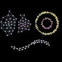
№ 1 Hasegawa SOINN. , . 10% . , , SOINN , . . . , , № 1 ( 1). .

1. № 1
2. ESOINN № 1
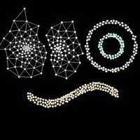
3. ESOINN № 1
ESOINN . λ=100, =100, c1=0.001 c2=1. 2 ; 3 . ESOINN . ESOINN SOINN .
№ 2 ( 4), , SOINN ESOINN. 10% . , , . . , , . 1. 10000 , 2. 10000 , 3 . , , .
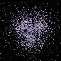
4. № 2
5. SOINN № 2
6. SOINN № 2
5 6 SOINN ( : λ=200, =50, c =1 , Shen, F., & Hasegawa, O. (2006a). An incremental network for on-line unsupervised classification and topology learning. Neural Networks, 19, 90–106.) SOINN .

7. ESOINN № 2

8. ESOINN № 2
7 8 ESOINN ( : λ=200, =50, c1=0.001 c2=1). SOINN, ESOINN . , . № 2 , ESOINN , SOINN.
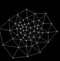
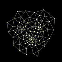
10 AT&T_FACE ; 10 ( 9). 92112 , 256 . . , 92112, 2328 . 2328 width=4, q=2 2328 ( 10)
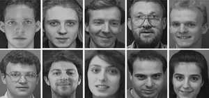
9.

10.
, . 1, 1000 , 2 . : λ=25, =25, c1=0.0 c2=1.0. , ESOINN 10 ( ) . . SOINN, (90% 86% ).
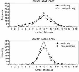
11.
SOINN ESOINN, 1000 . 11 SOINN, 11 – ESOINN. SOINN (2-16) , ESOINN (6-14); 10 SOINN ESOINN, , ESOINN , SOINN.
, Optical Recognition of Handwritten Digits database (optdigits) ( www.ics.uci.edu ˜mlearn/MLRepository.html ) SOINN ESOINN. 10 ( ) 43 , 30 13 – . 3823 , 1797 . 64.

12. . SOINN, ESOINN
-, SOINN ( λ=200, =50, c =1.0 ). SOINN 10 . , 12, SOINN. SOINN . 92,2%; 90,4%. 100 SOINN. 6 13 ( ).
ESOINN. (λ=200, =50, c1=0.001 c2=1), ESOINN 12 . 12 ESOINN. ESOINN 1 9 , 1 1' 9 9'. SOINN , 1' 9'. ESOINN 1 1' (9 9'), .
ESOINN . 94,3% 95,8%. 100 ESOINN. 10 13 .
, ESOINN , SOINN. ESOINN SOINN.
Conclusion
ESOINN, SOINN. SOINN, ESOINN . ESOINN () . ESOINN , . ESOINN . ESOINN SOINN. , ESOINN SOINN.
, Learning Vector Quantization (LVQ). . , . , , . ESOINN SOINN , , ESOINN . . ESOINN .
- ESOINN
ESOINN 1,8 . ( )
ESOINN , . .
Github SOINN ++ ( )
SOINN OpenCV ( SOINN )
SOINN is a self-organizing incremental neural network. The structure and algorithm of such a neural network seems to have worked well in the Japanese laboratory Hasegawa (site - haselab.info ), because it was eventually taken as a basis and the further development of algorithms of artificial intelligence went through small modifications and add-ins to the SOINN network.
The core network SOINN consists of two layers. The network receives the input vector and on the first layer after training creates a node (neuron) - the defining class for the input data. If the input vector is similar to the existing class (the measure of similarity is determined by the learning algorithm settings), then the two most similar neurons of the first layer are connected by a link, or if the input vector is not similar to one existing class, then the first layer creates a new neuron that defines the current class. Very similar neurons of the first layer, combined by a link, are defined as one class. The first layer is the input layer for the second layer, and according to a similar algorithm, with a few exceptions, classes are created in the second layer.
')
On the basis of SOINN such networks are created as (the network name and the description of the network from its creators are presented below):
ESOINN - expansion of the SOINN neural network is trained online without third-party intervention and without setting a learning task. This is an improved version of the SOINN network for on-line uncontrolled classification and training topology. 1 - this network consists of one layer as opposed to two layers in SOINN; 2 - its clusters with high density of overlap; 3 - it uses fewer parameters than SOINN; and 4 - it is more stable than SOINN. Experiments on demo data and real data also show that ESOINN works better than SOINN.
ASC data classifier based on SOINN. It automatically determines the number of prototypes and assimilates new information without deleting the information already stored. It is resistant to noisy data, the classification is very fast. In the experiment, we use both demo data and real data sets to illustrate ASC. In addition, we compare ASC with other results based on classifiers, taking into account its classification of errors, compression and speed of classification. The results show that ASC has better performance and is a very effective classifier ( Reference to the original ).
GAM - General Associative Memory (GAM) is a system that combines the functions of another type of associative memory (AM). GAM is a network consisting of three layers: an input layer, a memory layer, and an associative layer. The input layer accepts input vectors. A memory layer saves input to similar classes. The associative layer builds associative connections between classes. GAM can store and call binary or non-binary information, build many-to-many associations, store and recall both static data and a temporary sequence of information. May recall information even if it has incomplete input data or noisy data. Experiments using real-time binary data using static data and time sequence data show that GAM is an efficient system. In experiments using human-like robots, it demonstrates that GAM can solve real problems and build connections between data structures with different sizes ( Reference to the original ).
The new STAR-SOINN (STAtistical Recognition - Self-Organizing and Incremental Neural Networks) - to build a smart robot, we must develop the psychic system of an autonomous robot that consistently and quickly learns from man, his environment and the Internet. Therefore, we offer the STAR-SOINN network - this is an ultra-fast, multi-modal network that learns in real time and has the ability to additionally learn via the Internet. We conducted experiments to evaluate this teaching method and compared the results with other teaching methods. The result shows that recognition accuracy is higher than a system that simply adds conditions. In addition, the proposed method can work very quickly (for about 1 second to study an object, 25 milliseconds, for object recognition). The algorithm was able to identify the attributes of "unknown" objects by searching for the attribute information of known objects. Finally, we decided that this system potentially becomes the base technology for future robots.
SOIAM - modification SOINN for associative memory.
SOINN-PBR - modification of SOINN to create rules using conditions if -> then (if-then)
AMD (Autonomous Mental Development) - a robot using this algorithm to learn to solve various problems.
The block diagram of the SOINN algorithm can be found here.
A link to the magazine in pdf format, where a description of several SOINN networks in English is given and where I made notes in Russian (I packed the rar archive, the original magazine size was 20 mb ( read online ), the archive size was 13 mb ( download archive ).
Link to another magazine in pdf format, which describes several varieties of SOINN networks in English and where I made notes in Russian (I packed the rar archive, the original journal size was 4mb ( read online ), the archive size was 2.5mb ( download archive ).
In the Russian-language Internet about the SOINN network, there are only a couple of articles that the robot, working according to this algorithm, finds solutions to the problems and if it is not explained how to solve the problem, then it connects to the Internet and looks for a solution there. But I did not find examples of the operation of the algorithm and codes. Only there was one article on robocraft where a small example of the operation of the basic algorithm of the SOINN network in conjunction with OpenCV is given. If someone experimented with the SOINN network, it would be interesting to look at the code, if possible.
Back in 2006, a method of gradual (increasing) learning was proposed, called the self-organizing growing neural network (SOINN), in order to try to implement unsupervised learning (self-study without a teacher). SOINN does a good job of processing non-stationary data online, reports the number of defined clusters, and represents the topological structure of the input data, taking into account the probability of the probability distribution density. Hasagawa, who proposed a version of the SOINN network, compared the results of his network operation with the GNG network (expanding neural gas) and the result of the SOINN network was better than that of the GNG network.
There were such problems with the SOINN network:
1. Due to the fact that it consisted of two processing layers, that the user had to take part in the network. The user had to decide when to stop learning the first layer and when to start acquiring knowledge in the second layer.
2. If the groups have high density, then the network coped well with their recognition, but if the network of the group partially overlapped, then the network thought it was one group and united them.
To solve these problems and simplify the network architecture, a SOINN-based network with increased self-organization was proposed and called ESOINN.
SOINN Short Review.
Soinn consists of a network with two layers. The first layer studies the distribution density of the input data and uses the nodes and the connections between them to represent the result of the data distribution. The second layer searches for data in the first layer with the lowest distribution density and identifies groups for them and uses fewer nodes than the first layer to provide the topological structure of the data under study. When learning of the second layer is completed, SOINN reports the number of found groups and assigns the input data to the group most suitable for it. The first and second layers work on the same algorithm.
When the input vector is applied to the network, it finds the closest node (winner) and the second closest node (second winner) to the input vector. Using threshold similarity criteria, the network determines whether the input vector belongs to the same group as the winner and the second winner. The first layer of SOINN adaptively updates the similarity threshold for each node separately, because the criterion for the distribution of input data is not known in advance.
If a certain node i has neighboring nodes, then the similarity threshold Ti is calculated using the maximum distance between this node i and its neighboring nodes.
FORMULA 1A
Here, Ti (similarity threshold) is the distance to the most distant neighbor of node i. Wi is the weight of node i, Ws is the weight of neighboring node i
If node i does not have neighboring nodes, then the similarity threshold Ti is calculated as the distance between the vector i and the closest vector to it available in the network.
Formula 1B
Here, Wn is the weight of any host except the node i
If the distance between the input vector and the winner or the second winner is greater than the similarity threshold of the winner or the second winner, respectively, then the input vector is inserted into the network as a new node and now represents the first node of the new class. This insert is called an insert between classes, because this insert creates a generation of a new class, even if a new class can be classified in the future as any of the already existing classes.
If the input vector is defined as belonging to one cluster as the winner or the second winner, and if there are no links connecting the winner and the second winner, then connect the winner and the second winner using the connection and set the age of this connection to zero; further increase the age of all ties connected to the winner by 1.
Then we update the weight of the vector of the winner and his neighbors nodes. We use node i with input data to find the winner node and in the node variable — Win_Number — we show how many times node i was the winner.
Change the weight of the winner according to the formula:
Formula 1C
where Wwin is the winner's weight, Cwin is the number of victories of the winner, Wi is the weight of the input vector
Change the weights of all the neighbors of the winner according to the formula:
Formula 1D
where Wswin is the winner’s neighbor weight, Cwin is the number of victories won, Wi is the weight of the input vector
If the age of the connection between the nodes is greater than the preset parameter Maximal_expression_connection, then we delete this connection.
When, during the iterative network learning, the preset Time-of-Learning parameter has come to an end, then SOINN realizes that the time for learning is over, it inserts a new node to a point in the topological map, where the accumulated error is the longest. Cancel node insertion if the insert cannot reduce the size of the error. This insert is called an insert within the class because the insert occurs within the class. Also, no new class will be created during this insertion. Then SOINN finds nodes whose number of neighbors is less than or equal to one and removes such nodes, based on the assumption that such nodes lie in a region of low density. Such nodes are called noise nodes (noisy nodes).
In fact, because the similarity threshold of the first layer of SOINN is updated adaptively, the accumulation error will not be high. Therefore, an insert within a class is of little use. Insertion within the class for the first layer is not needed.
After the expiration of the iterative learning time of the first layer, the learning results of the first layer are fed as input to the second layer. The second layer uses the same learning algorithm as in the first layer. For the second layer, the similarity threshold (Ti) is constant. It is calculated using the distance within the class and the distance between the classes. With a large constant similarity threshold, unlike the first layer, the accumulated error for nodes of the second layer will be very high, and here the insertion within the class plays a big role in the learning process. With a large constant similarity threshold, the second layer can also remove some noisy nodes that remain unremoved during the training of the first layer.
The two-layer SOINN network has the following disadvantages:
It is difficult to choose when to stop learning the first layer and start learning the second layer;
If the results of the study of the first layer were changed, all the studied results of the second layer will be destroyed, thus reclassification of the second layer will be required. The second layer of SOINN is not suitable for gradual online learning.
Insertion within the class is necessary for the second layer, but it requires many user-defined parameters.
SOINN is unstable - it cannot separate high-density classes that partially overlap each other.
In order to get rid of the aforementioned drawbacks, the developers removed the second layer of SOINN and changed some methods to help a single layer get better classification results than a two-layer SOINN. Such a network is called ESOINN.
ESOINN accepts data on a single layer. For insertion between classes, the same algorithm is used as for SOINN. When creating a connection between the nodes, ESOINN adds the condition whether to create a connection.
After the expiration of the Timer_Tutorial timer, ESOINN separates the nodes into different subclasses and removes the links that lie in the overlapped areas. ESOINN does not use inserts within a class.
Removing the second layer makes ESOINN more suitable for continuous (incremental) online learning than double-layer SOINN. It also removes the difficulty of choosing when to finish the first layer and start the second layer. Refusal to insert within the class removes five parameters from the network that were necessary for the implementation of such an insert, and the understanding of the network operation algorithm is simplified.
ESOINN operation algorithm
Overlapping classes (partial superposition of classes on each other). Let us discuss how to determine the density of a node, using what method one can find the overlap of one class by another, whether it is necessary to build a connection between the winner and the second winner. The density of the spatial distribution of nodes in the overlapped region is lower than in the center of the class.
Knot density
The density of a node is determined by the local accumulation of the number of examples (input data). If there are many input samples near the node, then the density of the node is considered high, if the input examples near the node are not large, then the density of the node is considered low. Therefore, at the time when the network is studying, we must count how many times the node was the winner in the variable was the winner, which will show the density of this node. You can determine the density of a node by using an algorithm like SOINN. Here the following problems appear:
1. There will be numerous nodes that lie in areas of high density. In an area with a high density, the chance for a node to be a winner will not be significantly higher than in an area with a low density. Consequently, we cannot simply use a node's winner in order to measure its density.
2. In the growing tasks of learning, some nodes created at earlier stages will not be winners again over time. Using the definition of "winner", such nodes can be evaluated as low-density nodes at a later stage of training.
ESOINN uses a new definition of density to help solve the problems described above. The basic idea is the same as in the local accumulation of the number of input examples (data), but we define a “point” occupying the space of “numbers” and use the average of the accumulated points of a node to describe the density of this node. Unlike the winner, who binds himself to only one special node, the relationship between the nodes is considered here when we calculate the point P of the node. First we calculate the average distance.
node i from its neighbors.FORMULA 1
Where m is the number of neighbors of node i, Wi is the weight of vector of node i, Wj is the weight of vector of neighbor of node i
Then we calculate the POINT of the node i as follows:
Formula 2
if node i is the winner if node i is not a winnerFrom the definition of a POINT, we see that if the average distance from node i to its neighbors is large, then the number of nodes in this area is small. Consequently, the distribution of nodes is rare and the density in this area will be low. Thus, we give the low POINT to the node i. If the average distance is small, it means that the number of nodes in this area is high and the density in this area will be high. Therefore, we give a high POINT to the node i. For one iteration, we only calculate POINTS for node i, when node i is a winner. The POINTS of other nodes in this iteration are 0. Therefore, for one iteration, the accumulated POINTS of the winner will be changed, but the accumulated POINTS of the other nodes remain unchanged.
The accumulation of DOTS Si is calculated as the sum of DOTS for node i during its training period.
Formula 3
Here, sig is the number of input signals during one training period. n - shows the time of the training period (which can be calculated as LT / sig, where LT is the average total number of input signals).
Therefore, we take the average accumulated POINT (density) of node i
Formula 4
Here N represents the number of periods when the accumulated points of Si are greater than 0. Note that N is not necessarily equal to n. We do not use n to take the space N because, for increasing learning during a certain period of learning, the accumulated DOTS Si will be equal to 0. If we use n to calculate the average accumulated DOTS, then the density of some of the old nodes studied will decrease. Using N to calculate the average of accumulated DOTS, even during lifelong learning, the density of old studied nodes will remain unchanged if no new signals close to these nodes are applied to the system. However, for some applications it is necessary that the very old information studied was forgotten. In such cases, we must use n to take the space N. Thus, we can study new knowledge and forget very old knowledge. In order for all the learned knowledge to remain in the network, you need to take N to determine the density of the node.
Search for overlapping areas between classes.
Regarding the definition of density, the easiest way to find covered areas is to look for areas with a low density. Some methods, such as GCS and SOINN, use this technique to identify overlapped areas. However, this technique cannot guarantee that a region with a low density is precisely an overlapped region. For example, for some class that follows the Gaussian distribution, the density at the class boundary will be low. The overlay includes some of the boundaries of the overlapped classes. Therefore, the overlap density should be greater than in the overlapped boundary region. To solve this problem, ESOINN does not use the lowest density rule, but rather creates a new technique to find the overlapped area.
In SOINN, after a period of study, if there is overlap between the classes, all nodes of such classes are connected to form one class. Our goal is to find an overlapped area in a complex class (which includes many groups), to avoid building new connections between different classes, and thus effectively separate overlapped classes.
To detect an overlapped area, you first need to divide the complex class into several subclasses, using the following rule:
Algorithm 1. Division of the composite class into subclasses
1. We will call a node the vertex of a subclass if the node has a maximum local density. Find all the vertices in the complex class and give each vertex a different label.
2. We classify all other nodes with the same label of the subclass as at their vertices.
3. Each node lies in the overlapped area if the connected nodes have different subclass labels.
This method seems reasonable, but for the actual problem it will lead to several problems. For example, there are two classes in which the density distribution of nodes is not smooth, but rather similar to the presence of noise. With algorithm 1, these two classes will be divided into too many subclasses and many overlapping areas will be detected. You need to smooth the input data before dividing a complex class into subclasses.
Picture 1
In Figure 1, two non-smoothed input classes.
Take subclass A and subclass B from figure 1. Suppose that the density of the vertex of the subclass A is Amax, and the density of the vertex of the subclass B is Bmax. We merge subclasses A and B into one class if the following condition is met:
If a
Formula 5
Or
Formula 6
Here, the winner and the second winner lie in the overlap area between subclasses A and B. In fact, L is a parameter that belongs to [0,1] which can be calculated automatically using the threshold function.
Formula 7
Here
is the average density of nodes in the subclass.Formula 8
Here N is the number of nodes in subclass A.
Thus, by dividing a composite class into different subclasses and then combining them without overlapping the subclasses into one subclass, one can find an overlapped area within the composite class. After we find the overlapped area, we remove the bonds between the nodes that belong to different subclasses and separate the overlapping classes.
Algorithm 2. Creating links between nodes
1. Connect two nodes with a link if the winner and the second winner are new nodes (it is not yet defined to which subclass these nodes belong)
2. Connect two nodes with a link if the winner and the second winner belong to the same subclass.
3. If the winner belongs to subclass A, and the second winner belongs to subclass B. If formulas 5 and 6 are fulfilled, connect these nodes with a link and combine subclasses A and B. Otherwise, we will not connect these nodes with a link, and if the connection between these nodes is already exists, then delete it.
We use algorithm 2, if the winner and the second winner belong to different subclasses, ESOINN in this case gives the two nodes the opportunity to be connected by a link. We can do so in order to limit the effects of noise during the division of subclasses and try to smooth out the oscillations of the subclasses. Subclasses can still be related to each other (for example, subclass A and subclass B in Figure 1) if the two subclasses are erroneously divided.
Algorithm 2 shows that the result of ESOINN will be more stable than that of the SOINN network, because even with low overlap density, SOINN will sometimes separate different classes correctly, and sometimes will recognize different classes as one class. Using the smoothing method, ESOINN can stably separate such overlapped classes. ESOINN also solves the problem of excessive separation.
Node removal due to noise
To remove nodes caused by noise, SOINN removes nodes in regions with very low probable densities. SOINN uses the following strategy: if the number of input signals generated so far is a multiple of the parameter
, delete the nodes that have only one neighboring node or there are no neighboring nodes at all. For one-dimensional input data and a low noise data set, SOINN uses a local accumulation of the number of candidate node signals for deletion to control the deletion behavior. In addition, in the two-layer structure of the network SOINN, the second layer helps to remove nodes caused by noise.For ESOINN, we use almost the same technique of removing nodes as a result of noise, like that of SOINN. If the number of input signals generated so far is a multiple of the parameter
, then we delete such nodes whose topological neighbors have 2 or less than two (<= 2). The difference between ESOINN and SOINN is that we also remove nodes with two topological neighbors. We use local accumulation of POINT and various control parameters C1 (for two neighboring nodes) and C2 (for one neighboring node) to select the behavior of deleting nodes. , ESOINN , SOINN. SOINN . ESOINN, . 1 .1 2 . 1 5, 5 3, 3 2. 1 2 .
, . , . , . , . , SOINN.
3.
1. .
2. i . i Ci
3. , i. i.
4. 2 , .
, ESOINN
4. ESOINN
1. , . , ⊂×
2.
3. () a1 ( ) a2 :
ξ a1 a2
or , 2 . T 1 14. a1 1
5. 2 a1 a2.
) : a1 a2 , 0; a1 a2 , a1 a2 0.
) : a1 a2 , a1 a2.
6. 4.
7. 1
, 8.
and . i a1SOINN
and 9. ,
.10. λ:
) 1
) :
1. , a ,
, a. – .2. ,
, .3. , , .
11. , 3; , .
12. 2 .
, . . , λ . , . λ . , , . ; . , . . , . ; . , , .
ESOINN
.
№ 1 Hasegawa SOINN. , . 10% . , , SOINN , . . . , , № 1 ( 1). .
1. № 1
2. ESOINN № 1
3. ESOINN № 1
ESOINN . λ=100,
=100, c1=0.001 c2=1. 2 ; 3 . ESOINN . ESOINN SOINN .№ 2 ( 4), , SOINN ESOINN. 10% . , , . . , , . 1. 10000 , 2. 10000 , 3 . , , .
4. № 2
5. SOINN № 2
6. SOINN № 2
5 6 SOINN ( : λ=200,
=50, c =1 , Shen, F., & Hasegawa, O. (2006a). An incremental network for on-line unsupervised classification and topology learning. Neural Networks, 19, 90–106.) SOINN .7. ESOINN № 2
8. ESOINN № 2
7 8 ESOINN ( : λ=200,
=50, c1=0.001 c2=1). SOINN, ESOINN . , . № 2 , ESOINN , SOINN.10 AT&T_FACE ; 10 ( 9). 92112 , 256 . . , 92112, 2328 . 2328 width=4, q=2 2328 ( 10)
9.
10.
, . 1, 1000 , 2 . : λ=25,
=25, c1=0.0 c2=1.0. , ESOINN 10 ( ) . . SOINN, (90% 86% ).11.
SOINN ESOINN, 1000 . 11 SOINN, 11 – ESOINN. SOINN (2-16) , ESOINN (6-14); 10 SOINN ESOINN, , ESOINN , SOINN.
, Optical Recognition of Handwritten Digits database (optdigits) ( www.ics.uci.edu ˜mlearn/MLRepository.html ) SOINN ESOINN. 10 ( ) 43 , 30 13 – . 3823 , 1797 . 64.
12. . SOINN, ESOINN
-, SOINN ( λ=200,
=50, c =1.0 ). SOINN 10 . , 12, SOINN. SOINN . 92,2%; 90,4%. 100 SOINN. 6 13 ( ).ESOINN. (λ=200,
=50, c1=0.001 c2=1), ESOINN 12 . 12 ESOINN. ESOINN 1 9 , 1 1' 9 9'. SOINN , 1' 9'. ESOINN 1 1' (9 9'), .ESOINN . 94,3% 95,8%. 100 ESOINN. 10 13 .
, ESOINN , SOINN. ESOINN SOINN.
Conclusion
ESOINN, SOINN. SOINN, ESOINN . ESOINN () . ESOINN , . ESOINN . ESOINN SOINN. , ESOINN SOINN.
, Learning Vector Quantization (LVQ). . , . , , . ESOINN SOINN , , ESOINN . . ESOINN .
- ESOINN
ESOINN 1,8 . ( )
ESOINN , . .
Github SOINN ++ ( )
SOINN OpenCV ( SOINN )
Source: https://habr.com/ru/post/188230/
All Articles