Index the sky
The need for spatial search arises quite often. As well as in spatial JOIN'e - finding the intersection of two sets of features. Not always want to attract heavy artillery. Well, let's try to think of a way to solve the problem with “a little blood, a mighty blow”.
Introduction
It is known that indexing of more than one-dimensional objects is a significant problem, although the need for this is quite large. The difficulties are objective. whatever we do, the index file on the physical media is sequential (one-dimensional) and we must provide some sort of traversal order of the plane (space). At the same time, there is an intuitive desire to locate points in space that are not very far in the index file. Unfortunately, without breaks it is impossible.
The relationship to spatial indexing in the GIS community is generally twofold. On the one hand, a fair number of members of this community are confident that there is no problem and, should such a need arise, they would cope with it in two accounts. On the other hand, there is an opinion that “everything is already stolen before us”, most modern DBMS somehow know how to solve this problem, some for a long time and, in general, successfully.
')
As it often happens, the fact that we do not see a gopher does not mean that it is not there. As soon as the data volumes grow significantly, it is found that the construction of the spatial index itself can be a problem, since either the algorithm goes beyond the definition, or the construction time becomes unacceptably large, or the search is ineffective ... As soon as spatial data begins to change intensively, the spatial index may begin to degrade. Index rebuilding helps, but not for long.
Here we consider the simplest case of indexing spatial data - working with point objects. We will use honest coding of coordinates using a sweeping curve. Of course, there are other methods, pixel-block indices, R-trees, quadtrees, at worst. Perhaps this is a topic for another article, but now we are describing exactly how to work with point objects with the help of a sweeping curve.
We will not argue that the proposed method is ideal, but it has at least two advantages - it is very simple and very effective. With it, literally “on the knee”, it is possible to solve quite serious tasks.
We take the star atlas and its imitation with random numbers as data. Each data set consists of a number of objects, each of which is described:
- X - coordinate, 32-bit integer value
- Y - coordinate, 32-bit integer value
- VAL - 32 bit integer value
Test data
We have several data sets:
- 55M - This set consists of 55,368,239 objects whose coordinates are random numbers in the interval 0 ... 2 ** 27 in X and 0 ... 2 ** 26 in Y, VAL is always 0.
- 526M - This set consists of 526,280,881 objects whose coordinates are random numbers in the interval 0 ... 2 ** 27 for X and 0 ... 2 ** 27 for Y, VAL is always 0.
- USNO-SA2.0 - This is a directory of 55.368.239 stars, obtained from ftp://ftp.nofs.navy.mil .
X-coordinate is (RA (Right Ascension) in decimal hours) * 15 * 3600 * 100
Y - coordinate - ((DEC in decimal degrees) +90) * 3600 * 100
VAL - some value, which, among other things, contains the brightness in the red and blue ranges. - USNO-A2.0 - This is a directory of 526,280,881 stars, which can be obtained from ftp://ftp.nofs.navy.mil . For this data, only estimates are given. Values for its objects are similar to USNO-SA2.0
Theory
The idea of a sweeping curve is to number the discrete space. A feature is represented by a point in N-dimensional space. A point on the plane represents itself, a rectangular extent describing a flat figure is a 4-dimensional point, etc. Such a point is a fixed-length number that is fairly easy to deal with. In particular, such a number can be placed in a regular B-tree. The search query is divided into continuous segments of the sweeping curve and a subquery is executed for each segment. All points in the subquery intervals are the sought ones.
Thus, we need a curve that will visit every point of our (two-dimensional in this case) discrete space. What are the possible options?
- Igloo. 2-dimensional space is numbered line by line like a scan in a kinescope. For evenly distributed point objects in two-dimensional space and for small queries, this method is ideal. Its disadvantages are:
- Effectively works on 2-dimensional space, otherwise it generates a lot of subqueries.
- For large search extents, a large number of subqueries are generated.
- Ineffective for clustering-prone data.
- Effectively works on 2-dimensional space, otherwise it generates a lot of subqueries.
- Self-similar curves. The spotting curve has a fractal nature, the unit cell (for example, a 2x2 square) is numbered in a certain way, after which each sub-cell is numbered in a similar way. The most famous of such a curve is the so-called Z-order (or bit-interleaving), the nature of which follows from the name. The numbering of the plane with a resolution of 64x64 looks like:
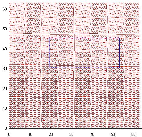
The blue rectangle in the picture is a typical search query, each time it crosses a curve, a new subquery is generated. In essence, with careless use, this method generates even more subqueries than igloo. This explains the fact that this method is practically not used in the DBMS. Although, self - similarity gives it a wonderful feature - adaptation to unevenly distributed data. In addition, continuous segments of the curve can cover large areas of space, which is useful if you are able to use it. - Another version of the self-similar curve: P-shaped Hilbert curve:
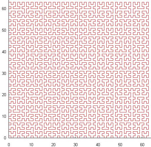
Unlike the Z-order, this curve has continuity, which allows searching a little more efficiently, a significant disadvantage is the relatively high cost of calculating coordinates from a value and vice versa.
The third variant with self-similarity 22: The X-shaped curve intersects itself and the author does not know the precedent of its use for spatial indexing.
Also known, the Moore curve is an analogue of the Hilbert curve, the Sierpinski curve, the Gosper curve, ... - We will use the so-called. Cascade Igloo:
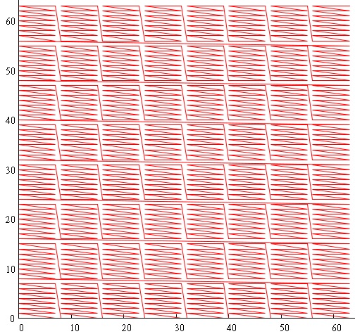
To get this picture, we divided the range of coordinates into pieces of 3 bits and mixed X & Y - i.e. the value of the sweeping curve is obtained as:- bits 0 through 3 are bits 0 through 3 x coordinates
- bits 3 through 6 are bits 0 through 3 Y coordinates
- bits 6 through 9 are bits 3 through 6 x coordinates
- bits 9 through 12 are bits 3 through 6 of the Y coordinate
But this is to demonstrate the principle. For indexing we will make blocks of 17 bits. If you are wondering why 17, more on that later.
results
Create index
| Dataset | Disk Size (Kb) | Build time | MEM size (Mb) |
|---|---|---|---|
| 55M | 211,250 | 6'45 " | 40 |
| 526M | 1,767,152 | 125 ' | 85 |
| USNO-SA2.0 | 376,368 | 4'38 " | 40 |
| USNO-A2.0 | 3,150,000 | 125 ' | 85 |
- Disk Size - the size of the resulting index file in kilobytes.
- Build Time - the time spent creating it in minutes / seconds
- MEM size is the peak size of RAM in Mb required by the index builder
Search index
The following tables list the values characteristic of queries on the constructed index. The total values for 100,000 searches for randomly selected (in a populated area, of course) square extents are given.
- 55M
Where:Extent Size Time (sec) NObj Rdisk σ (RDisk) 2x2 58 23 118,435 0.39 4x4 59 100 118,555 0.39 10x10 59 600 118,918 0.4 20x20 60 2,622 119,221 0.4 120x120 62 89,032 123,575 0.45 1200x1200 98 8,850,098 174,846 0.82 7200x7200 408 318,664,063 567,137 1.3 - Extent Size - search extent size, unit in case of USNO-SA (X) .0 is 1 arc second
- Time - time in seconds spent on executing 100,000 requests
- NObj - the number of objects found by all queries
- RDisk is the total number of disk read operations (misses by the internal cache), this value is much more indicative than time. even a file of hundreds of megabytes is effectively cached by the operating system
- σ (RDisk) - standard deviation of the number of disk operations, we note that according to the results of the experiments, the worst RDisk value did not exceed the average (RDisk) + 12 * σ (RDisk)
- 526M
Where the columns are similar to 55M.Extent Size Time (sec) NObj Rdisk 2x2 738 110 185,672 4x4 741 445 185,734 10x10 730 2,903 186,560 20x20 774 11,615 187,190 120x120 800 421,264 196,080 1200x1200 1200 42,064,224 307,904 7200x7200 3599 1,514,471,480 1,442,489
It is noteworthy that, while the number of disk accesses has changed slightly (by a third), query execution time has grown more than 10 times - the result of the lack of effective caching of the index file by the operating system. - USNO-SA2.0
Where the columns are similar to 55MExtent Size Time (sec) NObj Rdisk σ (RDisk) 2x2 48 28 143,582 0.5 4x4 50 115 143,887 0.5 10x10 45 657 144,085 0.5 20x20 45 2,585 144,748 0.51 120x120 47 94,963 151,223 0.56 1200x1200 80 9,506,746 224,016 0.97 7200x7200 387 345,165,845 842,853 2.97 - USNO-A2.0 (evaluation)
Where the columns are similar to 526MExtent Size Time (sec) NObj Rdisk σ (RDisk) 2x2 ~ 600 ~ 130 ~ 200,200 ~ 0.4 4x4 ~ 600 ~ 500 ~ 200,200 ~ 0.4 10x10 ~ 600 ~ 3,000 ~ 200,200 ~ 0.4 20x20 ~ 600 ~ 12,000 ~ 200,200 ~ 0.4 120x120 ~ 600 ~ 450,000 ~ 250,200 ~ 0.5 1200x1200 ~ 1,000 ~ 45,000,000 ~ 300,200 ~ 1.4 7200x7200 ~ 3500 ~ 1,600,000,000 ~ 1,500,200 ~ 2.0
Spatial JOIN
The following tables list the values characteristic of join'ov indexes. By join we mean the search for all objects located within a certain extent. For example, if the query parameter is 0.25 arc second, then for each element from one index a search will be performed in the second index with an extent of + - 0.25, i.e. square with sides 0.5x0.5 arc second and center at the reference point.
- USNO-SA2.0 vs USNO-SA2.0
Where:Extent Size Time (sec) NObj 0.5x0.5 175 2 2x2 191 410 6x6 212 4,412 - Extent Size - search extent in arc seconds
- Time (sec) - the request execution time in seconds
- NObj - the number of objects found (not including themselves), in this case it is necessary to divide in half because this is auto-join
- 55M vs USNO-SA2.0
Where columns are similar to USNO-SA2.0 vs USNO-SA2.0.Extent Size Time (sec) NObj 0.5x0.5 150 925 2x2 165 13,815 6x6 181 122,295 - 526M vs 526M
Where columns are similar to USNO-SA2.0 vs USNO-SA2.0.Extent Size Time (sec) NObj 0.5x0.5 1601 0 2x2 1813 916 6x6 2180 9943
How and why does it work?
For a start, we note the important points:
- For large files, disk caching does not work, you should not rely on it.
- The request processing time consists mainly of disk read times, everything else is relatively short.
- For randomly distributed queries, no caching works, if the index is arranged as a B-tree, you should not rely on the page cache and spend extra memory on it.
- For spatially close requests, a small (several dozen pages) cache is sufficient.
So, let's try to understand how the data is arranged.
- The global extent is 2 ** 26 X 2 ** 27 or 180X360 degrees.
- 180 degrees is 180 * 60 * 60 = 648,000 arc seconds.
- 1 << 26 = 67,108,864. This means that one angular second is ~ 100 counts.
- One object accounts for an average of 1600 = (2 * 648000 * 648000/500000000) square arc seconds ~ (40X40).
- Or 40 * 100 = 4000 counts.
- ~ 1000 objects are placed on the B-tree page.
- If we wanted to make the tree page commensurate with the cascade Igloo block, we would make this block of 4000 * sqrt (1000) => ~ 1 << 17
- That's the magic number 17.
- So, the average page has an extent of (40 * 32) ~ 1200X1200 arc-seconds.
- In the data, such a page is physically most likely located on two adjacent blocks of a cascade Igloo.
- Therefore, search queries of up to 600x600 angular seconds are likely to require only one reading of a leaf page.
- Given that the 4-level index tree and the upper two levels are effectively cached, an average query of this size requires two physical reads from the disk.
- What was required to explain.
So how is the search done?
- we cut the search extent into pieces according to the block index device.
- each extent portion corresponds to one index block and is processed independently.
- inside the block we find the boundaries of the search range
- subtract the entire range, filtering everything that falls outside the search extent.
Results
- Even the largest atlas of spatial objects known to us (~ 3,000,000,000 pieces) can be indexed in time, measured in hours.
- The amount of disk memory required to store such an index is measured in dozens (~ 30) gigabytes and is almost linear in the number of objects.
- The amount of RAM required for the search is very small (units of Mb), the index can be used, including in embedded systems
- For a spatial search along a small extent (the dimensions of which are comparable with the average distance between objects), the search time thus approaches the time of 2-3 disk operations, i.e. practically to the physical limit
- For relatively large queries, the search time depends more on the number of objects in the sample.
- In any case, the time remains predictable, which allows the use of this index, including in real-time systems
PS
The work described was carried out in 2004 in collaboration with Alexander Artyushin from the wonderful company DataEast . At that time, the author himself was an employee of this company and, yes, the publication is carried out with their consent, thanks to Evgeny Moiseyev emoiseev .
Iron in those days was not like the present, but the fundamental moments have not changed.
Source: https://habr.com/ru/post/186564/
All Articles