Pre-learning limited to Boltzmann machines for recognition of real images

Good day. This topic is designed for those who have an idea about restricted Boltzmann machine (RBM) machines and their use for pre-training neural networks. In it, we will look at the features of using limited Boltzmann machines for working with images taken from the real world, understand why standard types of neurons are poorly suited for this task and how to improve them, and also express some emotions on human faces as an experiment. Those who have no idea about RBM can get it, in particular, from here:

Implementing a Restricted Boltzmann machine on c # ,
Pre-training of the neural network using a limited Boltzmann machine

Why is everything bad

Limited Boltzmann machines were originally developed using stochastic binary neurons, both visible and hidden. The use of such a model for working with binary data is completely obvious. However, the vast majority of real images are not binary, but are represented at least by shades of gray with an integer brightness value of each pixel from 0 to 255. One of the possible solutions to the problem is to change the brightness values ​​so that they lie in the interval 0..1 (divide by 255 ), and we will assume that the pixels are actually binary, and the values ​​obtained represent the probability of setting each particular pixel to one. Let's try to use this approach for handwriting recognition ( MNIST ) and voila - everything works and works wonderfully! Why is everything bad?

And because in a set of real images the intensity of a certain pixel is almost always almost exactly equal to the average intensity of its neighbors. Therefore, the intensity should have a high probability of being close to the average and a small probability of being even a little distant from it. The sigmoidal (logistic) function does not allow achieving such a distribution, although it works in some cases where it does not matter (for example, handwritten characters) ^[1] .

How to make it good ...

We need a way of representing visible neurons, which is able to say that the intensity is most likely equal to, say, 0.61, less likely 0.59 or 0.63, and very very unlikely 0.5 or 0.72. The probability density function should look something like this:

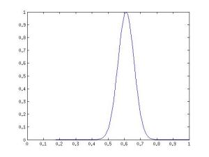
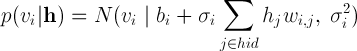
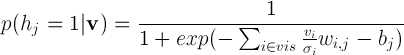
Yes, this is a normal distribution ! At least it can be used to model such behavior of neurons, which we will do by making the values ​​of visible neurons random variables with a normal distribution instead of a Bernoulli distribution . It should be noted that the normal distribution is convenient to use not only for working with real images, but also with many other data represented by real numbers from the range [-∞; + ∞], for which it does not make sense to reduce the values ​​to a binary form or probabilities from the range [0; 1] ^[2] . Hidden neurons remain binary and we get the so-called Gaussian-Binary RBM, the distribution of the values ​​of neurons for which are given by the formulas ^[3]
')





and the Boltzmann machine energy is equal



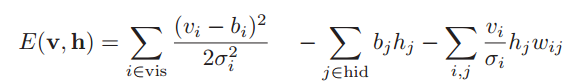
where hid is the set of indexes of hidden neurons,
vis - a set of indices of visible neurons,
b - bias (offset),
σ _i - the standard deviation for the i-th visible neuron,
w _{i, j} - the weight of the connection between the i-th and j-th neuron,
N (x | μ, σ ² ) is the probability of the value of x for a variable with a normal distribution with expectation μ and dispersion σ ² .

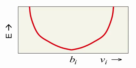
Let us consider how the RBM energy changes as v _i changes. Component b _i (bias) is responsible for the desired value of the i-th visible neuron (intensity of the corresponding pixel of the image), and the energy itself grows quadratically with a deviation from this value:

The last component of the formula, which depends both on v _i and h _i , and represents their interaction, depends on v _i linearly:

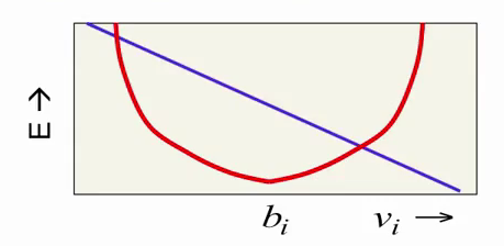
Summing up with a red parabola, this component shifts the energy minimum to one side or the other. In this way, we get the behavior we need: the red parabola attempts to limit the value of the neuron by not letting it move far from a certain value, and the purple line shifts this value depending on the hidden RBM state.

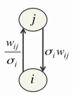
However, there are difficulties. Firstly, for each visible neuron, it is necessary to select the appropriate parameter σ _i as a result of training. Secondly, small values ​​of σ _i in themselves cause difficulties in learning, causing a strong effect of visible neurons on hidden and weak effects of hidden neurons on visible:


Thirdly, the value of the visible neuron can now grow indefinitely, causing the energy to fall indefinitely, which makes learning much less stable. To solve the first two problems, Jeffrey Hinton proposes to normalize all training data before starting training so that they have zero expectation and unit variance, and then set the parameter σ _i in the above equations to unity ^[4] . In addition, this approach allows using exactly the same formulas for collecting statistics and learning RBM using the CD-n method as in the usual case (using only binary neurons). The third problem is solved by simply reducing the learning rate by 1-2 orders of magnitude.

... and even better

As a result, we have learned how to represent real (valued) data with visible neurons of a limited Boltzmann machine, but the internal, hidden state is still binary. Is it possible to somehow improve the hidden neurons, to force them to carry more information? It turns out you can. It is very easy, leaving the hidden neurons to be binary, to make them display natural numbers greater than 1. To do this, take one hidden neuron and create many copies of it with exactly the same weigth sharing weights and learning from the bias b _i , when calculating the probabilities, we will subtract fixed values ​​from the displacement of each neuron, obtaining a set of otherwise identical neurons with offsets b _i -0.5, b _i -1.5, b _i -2.5, b _i -3.5 ... adding noise with variance σ (x) = (1 + exp (-x)) ^-1 (due to the probabilistic nature of the neurons). Simply put, the greater the value of x = b _i + ∑ v _j w _{i, j} at the input of such a neuron, the more copies of it are activated simultaneously, and the number of all activated copies will be the displayed natural number:



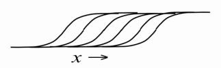
However, in reality, creating a large number of copies for each neuron is expensive, because it also increases the number of sigmoid function calculations at each iteration of the RBM training / work as many times. Therefore, we will act radically - we will create at once an infinite number of copies for each neuron! Now we have a simple approximation, which allows us to calculate the resulting value for each neuron by a single simple formula ^[1,5] :



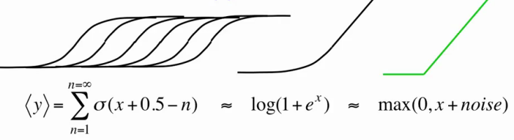
Thus, our hidden neurons were transformed from binary to rectified linear units with Gaussian noise, while the learning algorithm remained intact (after all, we assume that they are all the same binary neurons, with only an infinite number of copies described above). Now they are able to represent not only 0 and 1, and even not only natural, but all non-negative real numbers! The dispersion σ (x) ∊ [0; 1] ensures that completely inactive neurons will not create noise and the noise will not become very large with increasing x . In addition, a nice bonus: the use of such neurons still allows you to train the parameter σ _i for each neuron, if the preliminary normalization of data is for some reason impossible or undesirable ^[1,2] , but we will not dwell on this in detail.

Learning implementation

Taking the expectation from the formula of normal distribution, the value of the visible neuron can be considered by the formula


where N (μ, σ ² ) is a random variable with a normal distribution, expectation μ and dispersion σ ² .

Jeffrey Hinton in [4,5] suggests not to use Gaussian noise in reconstructions of visible neurons during training. Similar to the use of pure probabilities in the case of binary neurons instead of choosing 0 or 1, this speeds up learning by reducing noise and a bit less time for one step of the algorithm (do not count N (0.1) for each neuron). Following the advice of Hinton, we get completely linear visible neurons:



The value of the hidden neuron is calculated by the formula



To implement the learning itself, we use exactly the same formulas as for ordinary binary neurons in CD-n.

Experiment

As an experiment, we will choose something more interesting than simple recognition of faces or handwritten characters. For example, we will recognize which emotion is expressed on a person’s face. Use for training and testing images from bases
Cohn-Kanade AU-Coded Facial Expression Database (CK +) ,
Yale Face Database ,
Indian Face Database ,
The Japanese Female Facial Expression (JAFFE) Database .

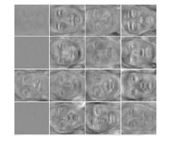
Of all the bases, we will only select images with a specific emotion (one of eight: neutral expression, anger, fear, disgust, joy, surprise, contempt, sadness). Get 719 images. 70% of randomly selected images (500 pieces) are used as training, and 30% of the remaining (219 pieces) as verification data (in our case they can be used as test ones, since we do not select any parameters with their help) . To implement we will use MATLAB 2012b. On each image, select the face using the standard vision.CascadeObjectDetector, expand the resulting square area down by 10% so that the chin fits completely into the processed image. The resulting image of the face will be compressed to a size of 70x64, translate into shades of gray and apply a histogram equalization to it to align the contrast on all images. After that, each image is expanded into a 1x4480 vector and store the corresponding vectors in the matrices train_x and val_x. In the matrices train_y and val_y, we save the corresponding desired vector-outputs of the classifier (size 1x8, 1 in the position of the emotion represented by the input vector, 0 in the remaining positions). The data is ready, it's time to start the actual experiment.

To implement the classifier, select the existing solution DeepLearnToolbox , fork, complete the functionality we need, fix bugs, shortcomings, inconsistencies with the Hinton guide and get a new DeepLearnToolbox , allowing you to simply take and use yourself for our task.

The number of neurons in each layer of our neural network: 4480 - 200 - 300 - 500 - 8. Such small numbers of neurons in hidden layers are selected in order to eliminate overfitting and simple memorization by the network of all input images, since their number is small. First, we will teach a neural network with a sigmoidal activation function, and for pre-training we use ordinary binary RBM.

tx = double(train_x)/255; ty = double(train_y); vx = double(val_x)/255; vy = double(val_y); % train DBN (stack of RBMs) dbn.sizes = [200 300 500]; opts.numepochs = 100; opts.batchsize = 25; opts.momentum = 0.5; opts.alpha = 0.02; opts.vis_units = 'sigm'; % Sigmoid visible and hidden units opts.hid_units = 'sigm'; dbn = dbnsetup(dbn, tx, opts); dbn = dbntrain(dbn, tx, opts); % train NN nn = dbnunfoldtonn(dbn, 8); nn.activation_function = 'sigm'; % Sigmoid hidden units nn.learningRate = 0.05; nn.momentum = 0.5; nn.output = 'softmax'; % Softmax output to get probabilities nn.errfun = @nntest; % Error function to use with plotting % calculates misclassification rate opts.numepochs = 550; opts.batchsize = 100; opts.plot = 1; opts.plotfun = @nnplotnntest; % Plotting function nn = nntrain(nn, tx, ty, opts,vx,vy); 

Neural Network Learning Schedule:


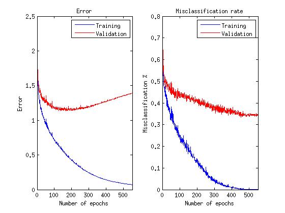
The average error on verification data among 10 launches with each time a new random sample of training and verification (validation) data was 36.26%.

Now we will teach the neural network with the rectified linear activation function, and for pre-training we use the RBM described by us.

 tx = double(train_x)/255; ty = double(train_y); normMean = mean(tx); normStd = std(tx); vx = double(val_x)/255; vy = double(val_y); tx = normalize(tx, normMean, normStd); %normalize data to have mean 0 and variance 1 vx = normalize(vx, normMean, normStd); % train DBN (stack of RBMs) dbn.sizes = [200 300 500]; opts.numepochs = 100; opts.batchsize = 25; opts.momentum = 0.5; opts.alpha = 0.0001; % 2 orders of magnitude lower learning rate opts.vis_units = 'linear'; % Linear visible units opts.hid_units = 'NReLU'; % Noisy rectified linear hidden units dbn = dbnsetup(dbn, tx, opts); dbn = dbntrain(dbn, tx, opts); % train NN nn = dbnunfoldtonn(dbn, 8); nn.activation_function = 'ReLU'; % Rectified linear units nn.learningRate = 0.05; nn.momentum = 0.5; nn.output = 'softmax'; % Softmax output to get probabilities nn.errfun = @nntest; % Error function to use with plotting % calculates misclassification rate opts.numepochs = 50; opts.batchsize = 100; opts.plot = 1; opts.plotfun = @nnplotnntest; % Plotting function nn = nntrain(nn, tx, ty, opts,vx,vy); 

Neural Network Learning Schedule:



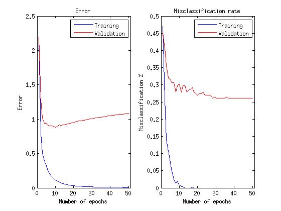
The average error on verification data among 10 runs with the same samples as for binary neurons was 28.40%

A note about graphs: since we are actually interested in the network’s ability to correctly recognize emotions, rather than minimize the error function, learning continues as this ability improves, even after the error function begins to grow.

As can be seen, the use of linear and rectified linear neurons in a limited Boltzmann machine made it possible to reduce the recognition error by 8%, not to mention the fact that it took 10 times less iterations (epochs) to train the neural network.

Links

1. Neural Networks for Machine Learning (video course)
2. Learning Natural Image Statistics with Gaussian-Binary Restricted Boltzmann Machines
3. Learning Multiple Layers of Features from Tiny Images
4. A Practical Guide to Training Restricted Boltzmann Machines
5. Recti fi ed Linear Units Improve Restricted Boltzmann Machines