Probabilistic models: the art of brackets
After a long break, we continue the cycle of graphical probabilistic models ( part 1 , part 2 ). Today, we are finally moving from problem statements to algorithms; let's talk about the simplest, but often useful algorithm for output on factor graphs - the message transfer algorithm. Or, as it can be called, the algorithm of correct placement of brackets.

by sergey-lesiuk
And let's start right away with a specific example - suppose you need to calculate the expression
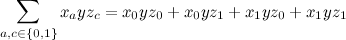
Here, formally speaking, there are four terms, each of the three factors, a total of three additions and eight multiplications.
')
Let's perform wonders of quick wits and note that the double sum here is decomposed into a product of two single sums:

Here suddenly there are only two additions and two multiplications - the benefit is evident. As you probably understand, if I was not too lazy to write a larger amount, the profit would have increased exponentially - we collapse the sum of the exponential number of the items into a product of a linear number of small brackets.
"Just think, binomial Newton!" - Readers will tell me; and they will be right, it really is very similar to Binom Newton. And attentive readers will also be surprised why there was a need for a little at all - indeed, in this example, it looks clearly superfluous.
Let's try to summarize the same example - now let some unknown function occur with our variables instead of multiplication:

Does the same trick pass above? No, it does not work out - we do not know any connection between different values of the function, it is a black box for us, and there’s nothing to put out of the bracket, we’ll have to honestly use the function four times and add the results.
The trick will take place in the intermediate case - we still leave in consideration a rather general function, but now we will assume that it decomposes into a product of a function of x and y and a function of y and z (finally, y will take part ):

With this formulation of the question, we can equally decompose a large amount into a product of two small ones:
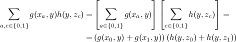
and save a lot on calculations. Note that although we assumed some additional structure for the function of three variables, it is not true that the variables x and z were completely independent in it - they were connected through y , which, by a happy coincidence, we did not need to summarize. By the way, notice that the result of this summation is a function of y .
What is the moral of this example? The fact that if we need to summarize a large function, and it decomposes into a product of smaller functions, it is possible that we can find a good decomposition into a product of parentheses ...
... but this is a withdrawal situation on a graphical probabilistic model! Recall the serial relationship between variables, which we discussed in the first series :
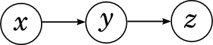
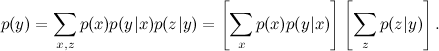
From a probabilistic point of view, it means that the joint distribution is decomposed as

And this means that the function of the three variables x , y and z is decomposed into the product of the function of x and y and the function of y and z , exactly as in our naive example. And the summation corresponds to the problem of marginalization : using this model and, possibly, the values of some variables, find the marginal probability distribution
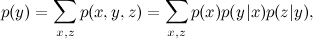
and we now understand that this expression can be significantly simplified as
The task of marginalization is the main one for graphic models, everything that we talked about last time is formalized through it: how to train regression weights, how to recognize speech using a ready-made model and how to train a recognition model from test examples, how to find players ratings after a regular tournament, how to find the extent to which topics enter documents from the corpus and so on.
The beauty of all this is that such reasoning does not need to be invented anew each time, but can be generalized. The most direct generalization is a chain of several events connected by a serial link:

At this place it will be convenient to change the picture a little. So far, we have drawn only variables, and the functions (probability distributions) were implied. In particular, it implied the expansion of a large function into factors; for example, the picture above leads to decomposition

Let's draw it now explicitly:

We have a bichromatic graph in which two types of vertices correspond to variables and functions. Each function is associated with those variables on which it depends, and the graph itself defines the decomposition of a large function into a product of small ones. This construction is called a factor graph - note that this is a more general construction than the Bayesian network of trust, now the probabilistic content is gone, and we can in principle speak about decomposing abstract functions (not necessarily distributions) into a product of smaller abstract functions (not necessarily conditional distributions).
Now let's apply our trick to the problem of marginalization with respect to x k . At first we bring in the first sum, then the second, then the third and so on until k -th; the result is a more compact representation of the left side of the summation, which, moreover, does not intersect with the right side (sorry for the long formula, but it is much more visual than the words here):
Similarly, you can do with the right side, and the result is
Pay attention to which calculation algorithm corresponds to our trick: we start from the edges of the graph (from the innermost brackets) and gradually go to the middle (more precisely, to the k -th variable), turning the sums on the way. This can be thought of as sending messages from the sides of the chain to the middle. At each step, we essentially do the same thing - we get the result of previous summations as a function of one variable h i ( x i ), and then we fold it with the following:

The general case of the message transfer algorithm is the case when the factor graph is a tree (that is, there are no cycles in it). In this case, you can prove that to marginalize for some vertex is enough:
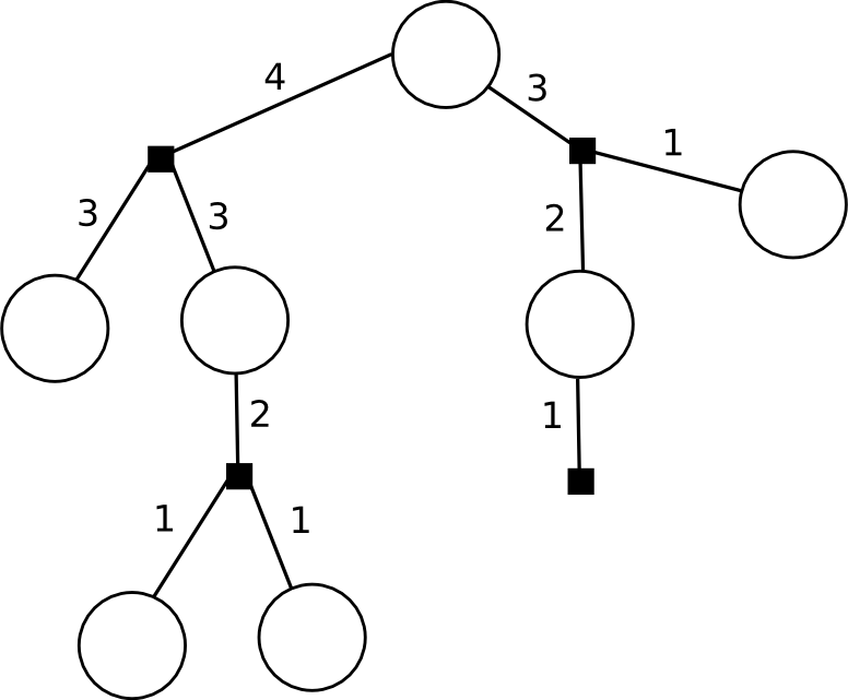
And to determine when it is already possible to transmit messages above, a very simple and comprehensive message passing rule is useful : the top of the factor graph can transmit a message to its neighbor if it has already received messages from all other neighbors . In particular, the leaves have only one neighbor, so they start sending messages there right away. This is how messages in a typical tree will go (the numbers indicate on which “tact” this message will be generated; we are now only looking at messages going from bottom to top).
The message that the variable node transmits is simply the product of all the messages it received (in the case of a sheet, the identity unit):
And in order to recount the message of a node-function, it is necessary to carry out a partial marginalization; if function already received messages
  from all variables
  , it can pass a message to the variable x

The function list, respectively, passes its own neighbor to itself (the product turns out to be empty). We assume here that each function involved in the decomposition depends on a sufficiently small number of variables so that these summations can be carried out by “brute force” (or at least somehow, if a particularly tricky case turns out).
The messaging algorithm works only when the factor graph is a tree. If there are cycles in the factor graph, the algorithm does not work (imagine that there is nothing but a cycle - then where to start?). However, in life very often there are situations when cycles are still present in the factor graph; for example, the LDA model for thematic modeling from the previous series generally consists of several almost complete bipartite graphs, each document is associated with each topic, there are continuous cycles in the factor graph.
Next time we will talk about what can be done in a situation when there are cycles in the graph. We are already approaching the border of what is possible, while remaining in our minds, to be explained in detail in a popular article intended for a wide audience, but I will try to give some intuition next time. And then, let's move on to specific examples.
by sergey-lesiuk
Example
And let's start right away with a specific example - suppose you need to calculate the expression
Here, formally speaking, there are four terms, each of the three factors, a total of three additions and eight multiplications.
')
Let's perform wonders of quick wits and note that the double sum here is decomposed into a product of two single sums:
Here suddenly there are only two additions and two multiplications - the benefit is evident. As you probably understand, if I was not too lazy to write a larger amount, the profit would have increased exponentially - we collapse the sum of the exponential number of the items into a product of a linear number of small brackets.
"Just think, binomial Newton!" - Readers will tell me; and they will be right, it really is very similar to Binom Newton. And attentive readers will also be surprised why there was a need for a little at all - indeed, in this example, it looks clearly superfluous.
Let's try to summarize the same example - now let some unknown function occur with our variables instead of multiplication:
Does the same trick pass above? No, it does not work out - we do not know any connection between different values of the function, it is a black box for us, and there’s nothing to put out of the bracket, we’ll have to honestly use the function four times and add the results.
The trick will take place in the intermediate case - we still leave in consideration a rather general function, but now we will assume that it decomposes into a product of a function of x and y and a function of y and z (finally, y will take part ):
With this formulation of the question, we can equally decompose a large amount into a product of two small ones:
and save a lot on calculations. Note that although we assumed some additional structure for the function of three variables, it is not true that the variables x and z were completely independent in it - they were connected through y , which, by a happy coincidence, we did not need to summarize. By the way, notice that the result of this summation is a function of y .
What is the moral of this example? The fact that if we need to summarize a large function, and it decomposes into a product of smaller functions, it is possible that we can find a good decomposition into a product of parentheses ...
To probabilistic models
... but this is a withdrawal situation on a graphical probabilistic model! Recall the serial relationship between variables, which we discussed in the first series :
From a probabilistic point of view, it means that the joint distribution is decomposed as
And this means that the function of the three variables x , y and z is decomposed into the product of the function of x and y and the function of y and z , exactly as in our naive example. And the summation corresponds to the problem of marginalization : using this model and, possibly, the values of some variables, find the marginal probability distribution
and we now understand that this expression can be significantly simplified as
The task of marginalization is the main one for graphic models, everything that we talked about last time is formalized through it: how to train regression weights, how to recognize speech using a ready-made model and how to train a recognition model from test examples, how to find players ratings after a regular tournament, how to find the extent to which topics enter documents from the corpus and so on.
Factor graphs and chain graph
The beauty of all this is that such reasoning does not need to be invented anew each time, but can be generalized. The most direct generalization is a chain of several events connected by a serial link:
At this place it will be convenient to change the picture a little. So far, we have drawn only variables, and the functions (probability distributions) were implied. In particular, it implied the expansion of a large function into factors; for example, the picture above leads to decomposition
Let's draw it now explicitly:
We have a bichromatic graph in which two types of vertices correspond to variables and functions. Each function is associated with those variables on which it depends, and the graph itself defines the decomposition of a large function into a product of small ones. This construction is called a factor graph - note that this is a more general construction than the Bayesian network of trust, now the probabilistic content is gone, and we can in principle speak about decomposing abstract functions (not necessarily distributions) into a product of smaller abstract functions (not necessarily conditional distributions).
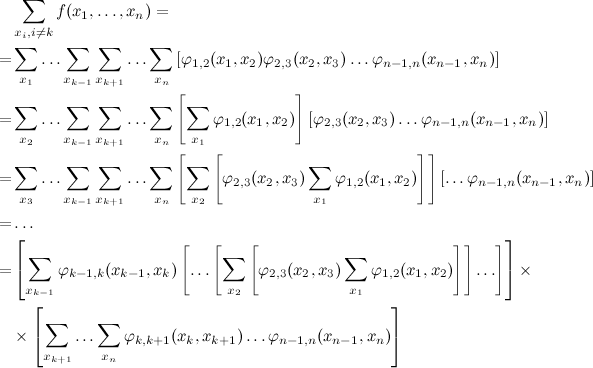
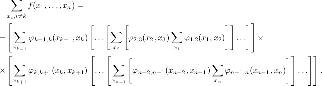
Now let's apply our trick to the problem of marginalization with respect to x k . At first we bring in the first sum, then the second, then the third and so on until k -th; the result is a more compact representation of the left side of the summation, which, moreover, does not intersect with the right side (sorry for the long formula, but it is much more visual than the words here):
Similarly, you can do with the right side, and the result is
Pay attention to which calculation algorithm corresponds to our trick: we start from the edges of the graph (from the innermost brackets) and gradually go to the middle (more precisely, to the k -th variable), turning the sums on the way. This can be thought of as sending messages from the sides of the chain to the middle. At each step, we essentially do the same thing - we get the result of previous summations as a function of one variable h i ( x i ), and then we fold it with the following:
General case
The general case of the message transfer algorithm is the case when the factor graph is a tree (that is, there are no cycles in it). In this case, you can prove that to marginalize for some vertex is enough:
- consider this vertex as a temporary root of a tree;
- transmit messages from the leaves towards the root; each message is a function of exactly one variable - the one that is adjacent to the edge along which this message goes;
- multiply all messages that came to the root.
And to determine when it is already possible to transmit messages above, a very simple and comprehensive message passing rule is useful : the top of the factor graph can transmit a message to its neighbor if it has already received messages from all other neighbors . In particular, the leaves have only one neighbor, so they start sending messages there right away. This is how messages in a typical tree will go (the numbers indicate on which “tact” this message will be generated; we are now only looking at messages going from bottom to top).
The message that the variable node transmits is simply the product of all the messages it received (in the case of a sheet, the identity unit):
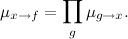
And in order to recount the message of a node-function, it is necessary to carry out a partial marginalization; if function
already received messages from all variables , it can pass a message to the variable xThe function list, respectively, passes its own neighbor to itself (the product turns out to be empty). We assume here that each function involved in the decomposition depends on a sufficiently small number of variables so that these summations can be carried out by “brute force” (or at least somehow, if a particularly tricky case turns out).
Conclusion and announcement of the next series
The messaging algorithm works only when the factor graph is a tree. If there are cycles in the factor graph, the algorithm does not work (imagine that there is nothing but a cycle - then where to start?). However, in life very often there are situations when cycles are still present in the factor graph; for example, the LDA model for thematic modeling from the previous series generally consists of several almost complete bipartite graphs, each document is associated with each topic, there are continuous cycles in the factor graph.
Next time we will talk about what can be done in a situation when there are cycles in the graph. We are already approaching the border of what is possible, while remaining in our minds, to be explained in detail in a popular article intended for a wide audience, but I will try to give some intuition next time. And then, let's move on to specific examples.
Source: https://habr.com/ru/post/185622/
All Articles