Digital Smoothing

Introduction

This article made me write a post habrahabr.ru/post/183986 , where it is not quite correct to use some kind of image smoothing algorithm.

Go right to the point.

Mathematical models of digital signals - vectors and matrices, whose elements are numbers. Numbers can be binary (binary signal), decimal ("normal" signal) and so on. Any sound, any image and video can be converted into a digital signal ¹ : sound into a vector, an image into a matrix, and video into a sequential set of matrices. Therefore, a digital signal is, one may say, a universal object for the presentation of information.
')
The task of smoothing is, in fact, the task of filtering a signal from stepwise (stepwise) changes. It is believed that the useful signal does not contain them. The stepped signal due to the set of sharp, but small in amplitude, level drops contains high-frequency components that are not present in the smoothed signal. Therefore, for some smoothing algorithm, it is first necessary to determine how different frequency components are attenuated. In other words, it is necessary to construct the amplitude-frequency characteristic of the corresponding filter, otherwise the probability of “running into” the artifacts is great.

The smoothing task can be used when thinning signals, that is, when, for example, you need to display a large image on a small screen. Or when the sampling rate of sound is reduced, for example, from 48000 Hz to 44100 Hz. Reducing the sampling rate is an insidious operation that requires preprocessing of the signal (low-pass filtering), but this is a topic for another conversation ...

Let's give an example of “bad” anti-aliasing.


It would seem that the usual averaging and the output signal should be “smooth”. But how to determine how he became "smoother"? Did we overdo it? Or maybe some coefficients are not chosen by 1/3? Or maybe averaged over five points? How to determine how attenuated the frequency components in the signal? How to find your (that is, for a specific task) optimum?
I will try to answer these and some other questions in such a way that the “ordinary” programmer can substantiate his algorithm - I hope not only the algorithm on the topic “Smoothing”, as the ideas will be presented very general, forcing you to think for yourself ...

Signals

In this paragraph, a signal is a vector, that is, an array of a certain number of numbers. For example, a vector of four elements s = (2,5; 5; 0; -5).

For simplicity, only decimal real numbers will be considered.

One of the most common and clear signals is the digitized sound. The size of the signal depends on the duration of the sound and on the frequency with which the samples are taken (on the sampling frequency). Elements-signal numbers depend on the current amplitude of the sound measured by the sampling and storage device.

As already mentioned, one of the easiest ways to smoothing is
(one)
where s is the original signal, v is the smoothed signal.

Method (1) is based on the smoothing property of summation, because it is clear to everyone that the average value, calculated as the sum of many random numbers, with increasing number of summed numbers becomes less and less similar to random variable ² , which, simply speaking, is noise ³ .

But what is the basis of the choice of coefficients in equation (1)? On the fact that the mean is calculated? It seems to be yes, but ... And if you take not three items, but sixteen? And thirty-two? .. Why are the samples more and more distant from the central element s [i] taken with the same weight? After all, it may be that the relationship between readings will gradually weaken with increasing distance ⁴ between them?

If we consider the example of the pronunciation of the word "watermelon" ten times in a row and try to track the relationship between the samples of the recorded signal, we can find a weakening of the dependence between the more and more distant samples. Naturally, if we consider the “long distances”, the sounds will be repeated by repeating the same word and the dependence will increase and decrease again, and so on. But, as a rule, “long distances” are not considered when smoothing, since noises appear in the vicinity of individual sounds, and not words, phrases and sentences. Noise acting at the level of words or even phrases is clearly artificial (sound effects) or exotic natural (echo). This is already "non-random" noise, which requires a separate study. Here we consider “pure” noise, which, to put it in simple terms, is annoyingly noisy and in no way resembles any useful signal.

Based on simple reasoning, it becomes obvious that the number of terms in (1) (the order of the filter) should depend on how strongly the neighboring samples depend on each other. For example, it makes no sense to take a filter of the thirtieth order, if only ten counts are observed, following each other. In fact, it’s not even that “there’s no point”, but it’s impossible, because if the samples are practically unrelated, then an excessive smoothing of the useful signal will begin (“devouring” syllables). But the third-order filter here will not be optimal in the degree of use of information about the useful signal, since, as already mentioned, there is a dependence of about ten neighboring samples. Therefore, you can “try your luck” with the help of a ninth-order filter, naturally, increasing the load on the processor-calculator. Here it is necessary to determine, most likely experimentally, and is this game worth the candle? ..

How to assess how closely related the next samples? Calculate the autocorrelation function (ACF). Those who wish can suggest experimenting on the recording of different words, phrases, repeating phrases and the subsequent construction of the ACF (since, for example, the Matlab program allows you to do this without particularly thinking about the code and formulas).

So how do you choose the filter coefficients in (1)?

In this case, it is convenient to consider the response of the filter to a single impact, that is, to a signal of the form


For example, the filter (1) will give the following response (impulse response)

whence we can conclude that after smoothing the duration of the signal became equal to three elements. And if you take a filter of five elements? .. Correctly, the duration of the output signal will be equal to five elements. How useful this is is determined by the specific situation (task).

By the way, the long-awaited artifact is already there! The impulse response (1) is, in fact, a rectangular impulse that is not at all smooth! .. Strange, yes? And if you take a five-point filter? Then at the output we get a longer rectangular pulse, but with a smaller amplitude. It doesn't work out very well ... The simplest test speaks of the unsuitability of simple averaging for smoothing.

Let's look at the filter (1) from the frequency side (we have already looked at the time line).

If the signal is sound, then it is quite well described by a set of harmonic signals ⁵ (“sinusoids”) and the degree of attenuation of a specific sinusoid depends on its frequency. Again, with proper selection of a smoothing filter, none of the useful sinusoids should disappear completely, that is, the amplitude-frequency characteristic of the filter in the operating frequency range should be fairly uniform.

Let us pass one single-tone signal of a certain frequency through the filter in question, of course, without going beyond the limits of the sampling theorem. Let the time discretization step T _d be equal to one, that is, the samples go in steps of one second. Take a signal with frequency f = 1 / (3 T _d ) = 1/3 Hz, i.e.


Confine ourselves to two periods


The response of the filter (1) will be equal to


Strangely enough, they got almost zero ... It turns out that some components of the useful signal can be lost.

Check the response to a slightly higher frequency signal.


As you can see, the shape of the signal is not lost. What's the matter? ..

The point is that the amplitude-frequency characteristic of the filter (1) is not monotonous in the working frequency band (in the range from zero to half of the sampling frequency) and has one zero at a frequency three times lower than the sampling frequency. How to show it?

Simply put, to determine the frequency response of the filter, it is necessary to find the ratio of the spectrum at the output of the filter to the spectrum at the input.

Denote the spectrum of the signal s [ i ] at the input as S ( f ), then the spectrum of the signal s [ i -1] delayed by one cycle T _d is expressed through the spectrum of the original signal as
(2)
where j is the imaginary unit.

The spectrum of the advanced signal s [ i +1] is expressed as
(3)

What does imaginary unit mean? And how can you justify (2) and (3)?
If we write the known [1, 2] series for sine, cosine and exponent
(four)
then by choosing the number j , such that j ² = –1, the last row can be expressed through the first two
(five)
which means that any complex number can be written through an exponent with an imaginary index. The modulus of the number (5) is equal to one (the square root of the sum of squares of the imaginary and real parts), therefore, to write any complex number in the form (5), it must be divided and multiplied by its own module
(6)

From (5) and (6) it follows that if in the exponent we can select an imaginary unit multiplied by a real number, then this number is an argument of a complex number.

In this case, the signals are considered, therefore the modulus of a complex number corresponds to the amplitude of the harmonic signal, and the argument is the phase. If, for example, take a signal of the form
(7)
then we can distinguish the amplitude A and the phase F. The multiplier - It is also a phase, and in some cases it is taken out of the brackets. For example, when passing a signal (7) through a filter, it is important to know the phase difference between the signals at the input and output, which the filter introduces at a given frequency f .

If the signal (7) is delayed by the value of t ₀ , then the same signal will be obtained, but shifted in phase by a constant value
(eight)
that is, when an arbitrary signal is delayed, all its frequency components are shifted in phase by an amount depending on the current frequency and the delay value. This may explain formulas (2) and (3). Therefore, when analyzing any algorithm, the phase-frequency characteristic is also important, which shows how long the filter (algorithm) delays each frequency component of the input signal. Low frequencies and high frequencies will generally have a different delay in the filter.

From (1), (2) and (3) it follows that the frequency response of the filter (transfer function) will be
(9)

Since the spectrum of the output signal is linearly expressed through the spectrum of the input signal, then at the output (9) the spectrum of the input signal is successfully reduced. Further, we note that the frequency response of the filter (1) is real, that is, this filter does not introduce phase distortion ⁶ . We achieved this (most likely, unconsciously) due to the symmetry of formula (1): each count at the output of the filter is equal to the sum of the current and two adjacent samples.

Physically, such an algorithm is realizable only in the presence of storage devices, since it uses advance readings (to calculate the readout s [ i ], the readout s [ i +1] is required). Currently, this is not a big problem and, as a rule, use symmetric algorithms. If phase distortions will be useful, then - please, the main thing is to consciously apply any algorithm and look at it from different angles: from frequency and time.

It is easy to build a graph of dependence (9) on frequency. For simplicity, the normalized frequency f ₀ = f T _d is entered, the useful range of which is [0 ... 0.5]. Signal components with frequencies above half the sampling frequency should be absent according to the sampling theorem (before digitizing, the signal is passed through the appropriate low-pass filters). The sampling rate indicates the number of readings by the digital device per second. If, for example, one clock cycle T _d is equal to one millisecond, then a thousand samples should be returned in one second.

Analyzing (9) it can be noted that the transmission coefficient is at a certain interval less than zero, and the amplitude is by definition a positive quantity ... The way out is to build the transfer function modulus by removing the minus sign in the phase characteristic, which, nevertheless, is not a constant (zero). If we take the number "minus one", then it can be represented by the formula (5) as
(ten)
that is, a complex number having the unit “unit” and the phase “180 degrees” (“pi”).

Thus, the three-point symmetric algorithm (1) for some “high” frequencies introduces a phase shift of 180 degrees, that is, it simply inverts the input signal. This effect can be noticed by analyzing the response considered above to the normalized frequency of 2/5 Hz.


Fig. 1. Amplitude-frequency and phase-frequency characteristics of a three-point symmetric smoothing algorithm (1)

From fig. 1 immediately follows that a signal with a frequency of 1/3 will be suppressed by this algorithm, and signals having a frequency higher than 1/3 will be inverted. Thus, the useful working frequency range can be safely reduced from [0 ... 0.5] to [0 ... 1/3]. If we are not satisfied with the rapid decay of the transmission coefficient, we will have to determine another algorithm that has a more rectangular amplitude-frequency characteristic and, at the same time, it is not yet known what phase ...

In essence, the obtained non-monotonic frequency response is a consequence of the rectangular shape of the impulse response ..., 0, 0, ..., 1/3, 1/3, 1/3, 0, 0, .... Therefore, the impulse response is an easy way to notice gross flaws in the algorithms. The frequency response, despite some difficulty in calculating it, is convenient in that it allows you to notice and correct more subtle flaws than we do.

If we now write algorithm (1) in a more general form
(eleven)
then, based on the knowledge of the frequency response, you can try to choose the coefficients so
so that the amplitude-frequency characteristic becomes monotonous in the working frequency range (0 ... 0.5). For this, at least, the absence of zeros within the working range is necessary.

Since we have no reason to single out the delayed reading s [i – 1] with respect to the leading s [i + 1], we equate the coefficients a ₁ and a ₃ . After we write down the transfer coefficient
(12)

We will try to move the first zero to the frequency f ₀ = 0.5. For this, the equality a ₂ = 2a ₁ must be satisfied, that is, the weight of the side samples must be two times less than the weight of the central one. Then a more optimal algorithm will look like this.
(13)

How to choose in (13) a single coefficient a ₁ ?

Let's look at algorithm (13) from the point of view of the impulse transient characteristic . For this we find the response to a single jump :
(14)

As you can see, in order to maintain the output amplitude in the steady state, equal to one, you need to choose the coefficient a ₁ = 1/4. That is, the sum of all coefficients must be equal to one.

Finally, for the finished algorithm
(sixteen)
You can build (Fig. 2) frequency characteristics: amplitude and phase.


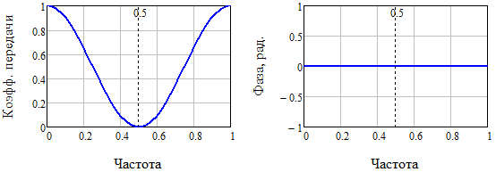
Fig. 2. Amplitude-frequency and phase-frequency characteristics of a three-point symmetric smoothing algorithm (16)

Analysis of fig. 2 shows that the phase distortions have disappeared, and the amplitude characteristic has become monotonous in the working frequency band [0 ... 0.5]. In a sense, we squeezed out of the three-point filter "everything".

Now it becomes obvious that simple averaging is by no means always optimal, especially when there are a lot of averaged samples.

Images

As for the images, here to some extent everything is the same as for the signals: amplitude and phase distortions, impulse characteristics, signal energy, the main difference is that matrices are used instead of vectors. It should also be noted that for images there is no time coordinate, but there is a coordinate of space, therefore there are spatial sampling rates. This difference is rather formal, since it does not affect the mathematics of algorithms at all.

Let us now consider the “simplest” algorithm for smoothing an image by neighboring points (Fig. 3). Count v ₀₀ at the output of the filter
(17)


Fig. 3. Scheme of smoothing the image by neighboring points

In formula (17), the three terms A , B, and C are specially distinguished, since the four corresponding internal terms of B and C have their own distances from the central reference s ₀₀ . It is natural to assume here that the maximum weight will be for the term A , then in descending order - for B and C.

For images, the spectrum and transmission coefficient will be two-dimensional, that is, they will depend on two frequencies: the first frequency - horizontally, the second - vertically (everything is conditional here, for definiteness).

The filter (17) has the following transfer coefficient
(18)

If we take, for example, about thirty discrete frequencies and construct (Fig. 4) a contour plot of the frequency response module (18), then we can see distortions similar to those in Fig. 1. The bottom left corner correspond to the lowest frequencies. There is a failure of the frequency response at frequencies that are 1/3 of the sampling frequency (in this case, the sampling frequency is 64 in both coordinates).


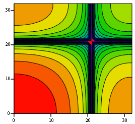
Fig. 4. Amplitude-frequency characteristic of nine-point symmetric smoothing algorithm (17)

Shuffling coefficients for samples in Fig. 3, you can get the following smoothing algorithm
(nineteen)

And if a single impact is placed in the center of the image, then the response of the filter (19) will look like
(20)

In fact, (20) is the impulse response of the filter (these are the nine main samples, since the others are zero). The sum of all counts of the impulse response is equal to one. The frequency response of the filter (19) has the form shown in Fig. five.


Fig. 5. Amplitude-frequency characteristic of nine-point symmetric smoothing algorithm (19)

Again we see (compare Fig. 4 and Fig. 5) the improvement of the ordinary averaging algorithm.

Summary

When developing digital signal processing algorithms (smoothing and not only) one should not trust intuitive algorithms like simple averaging.

A more general approach is the weight summation technique (only linear algorithms were considered, when samples are only multiplied by constants, and the results are added).

Weight summation, when weights are placed more distant from the central element of the readings, is justified both statistically (the natural nature of the weakening of dependence with distance) and functionally (it is possible to choose coefficients strictly mathematically, ensuring the monotonicity of the amplitude-frequency characteristic).

A large role is played by the amplitude-frequency characteristics of the filters, which are determined by the weighting sum coefficients. They allow us to prove that a given filter passes a certain frequency range and blocks another. Moreover, it is possible to determine the unevenness in the passband, in the stopband, and so on. The greater the order of the filter, the more degrees of freedom and the better you can choose the shape of the amplitude-frequency characteristic.

An important role is played by the phase-frequency characteristics, which are mainly determined by the degree of symmetry of the algorithm. Real-time algorithms, when the countdown at the filter output appears at the moment of arrival of the first sample, cannot provide a uniform phase response (constant, most often “zero”), since they cannot be symmetrical. Such algorithms introduce a delay into the input signal: for example, a smoothed image can generally shift along both coordinates. If the image is complex (that is, it has many frequency components), then its phase distortions can distort it noticeably, and not just shift it along the coordinates, which is approximately true for simple images.

You should also pay attention to the impulse response of the filter corresponding to a certain algorithm.This allows a simple way to look at the operation of the filter directly, that is, in the time scale for the signal or in the scale of spatial coordinates - for the image.

And finally, an energy analysis of the algorithm is needed, which allows determining the signal loss at the output of the corresponding filter. This analysis is conveniently carried out within the framework of the impulse transient response.

Footnotes

1. Always with losses, since the frequency of operation and the digit capacity of digital devices are limited
2. The average stabilizing property is valid if the characteristics of the random number generator are constant, that is, ideally, the generator should produce a random value with a given distribution law
3. If, of course, the observed noise - this is not an encrypted useful signal, which becomes random for those who do not have a key ...
4. For a sound signal, the distance between samples is a certain time interval
5. We can assume that any oh signal can be represented as a sum of sinusoids of multiple frequencies, but sound in nature is obliged to "well" decompose in a series of frequencies
6. Simplifiedly, you can say so, for details see below

Sources

1. Trigonometric functions [Electronic resource], access mode: free, ru.wikipedia.org/wiki/%D2%F0% E8% E3% EE% ED% EEC% E5% F2% F0% E8% F7% E5 % F1% EA% E8% E5_% F4% F3% ED% EA% F6% E8% E8
2. Exhibitor [Electronic resource], access mode: free, ru.wikipedia.org/wiki/%DD%EA%F1% EF% EE% ED% E5% ED% F2% E0