SMS filtering of spam using a naive Bayes classifier (R code)

Hey. In this post, we will look at a simple spam filtering model using a naive Bayes classifier with blur according to Laplace , write a few lines of code in R , and finally test it on an English-language sms spam database . Generally, on Habré, I found two articles on this topic, but none of them had a vivid example, so that you could download the code and see the result. There was also no mention of blur, which significantly increases the quality of the model, without much effort, unlike, say, a complex text preprocessing. But in general, the next post about naive bayes made me feel that I was writing a training manual for students with R code examples, so I decided to share the info.

Naive Bayes Classifier

')

Consider the set of some objects D = {dq, d2, ..., dm} , each of which has a certain set of features from the set of all features F = {f1, f2, ..., fq} , as well as one label from the set of tags C = {c1, c2, ..., cr} . Our task is to calculate the most probable class / label of an incoming object d, based on the set of its attributes Fd = {fd1, fd2, ..., fdn} . In other words, we need to calculate such a value of the random variable C , at which the a posteriori maximum (MAP) is reached.

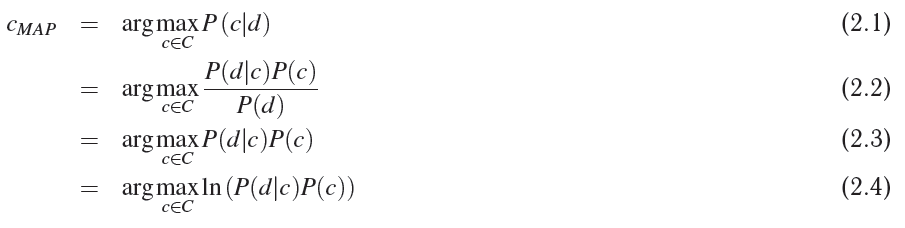
• 2.1 - in fact, this is our goal
• 2.2 - decomposed by the Bayes theorem
• 2.3 - given that we are looking for an argument that maximizes the likelihood function, and the fact that the denominator does not depend on this argument and is a constant in this case, we can safely delete the value of the total probability P (d)
• 2.4 - since the logarithm monotonously increases for any x> 0 , the maximum of any function f (x) will be identical to the maximum ln (f (x)) ; this is necessary so that in the future, during programming, not to operate with numbers close to zero

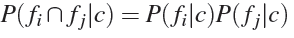
The model of the naive Bayes classifier makes two assumptions, from which it is so naive:

1. the order of the signs of the object does not matter;
2. probabilities of attributes are independent of each other for a given class: .

Given the above assumptions, we continue to derive formulas.

• 2.6-2.7 - this is just a consequence of the application of assumptions.
• 2.8 - here, just, the remarkable logarithm property is used, which allows us to avoid loss of accuracy when operating with very small values

We can depict a graphical model of a naive Bayes classifier as follows:

Spam classifier

Now, from the more general classification task, we dive into the specific task of classifying spam. So, the coupon D consists of SMS messages. Each message is marked with a label from the set C = {ham, spam} . In order to formulate the concept of signs, we will use the model of representation bag of words , we illustrate this with an example. Suppose we have only two ham sms messages in the database



hi how are you

how old are you



Then we can build a table

Word	Frequency
hi	one
how	2
are	2
you	2
old	one

There are only 8 words in the body of non-spam messages, then after rationing we get the a posteriori probability of the word using maximum likelihood estimation . For example, the probability of the word "how", provided that the message is not spam, will be:



P (fi = "how" | C = ham) = 2/8 = 1/4



Or we can write this method in general:



where q is the total number of unique words in the dictionary.

Laplace Blur

At this point, it's time to pay attention to the following problem. Recall our base of two ham messages, and, let's say, a message came to us for classification: " hi bro ", and, let's say, the a priori probability of non-spam P (ham) = 1/2 . Calculate the probabilities of words:

1. P ("hi" | ham) = 1/8
2. P ("bro" | ham) = 0/8 = 0

Recall formula 2.8 and calculate the expression under argmax with c = ham :





Obviously, we get either an error or a negative infinity, because the logarithm at zero does not exist. If we did not use logarithmization, then we would simply get 0, i.e. the probability of this message would be zero, which in principle gives us great benefit.



This can be avoided by Laplace blur or k-additive smoothing - this method allows you to blur when calculating the probabilities of categorical data. In our case, it will look like this:



, where z> = 0 is the blur coefficient, and q is the number of values ​​that a random variable can take, in our case it is the number of words in the class; and q is the total number of words that were used in teaching the model.



For example, when reading ham and spam messages, we found 10 unique words, then P ("hi" | ham) = (1 + 1) / (8 + 1 * 10) = 2/18 = 1/9 with a blur factor z = 1. And the zero probability ceases to be such: P ("bro" | ham) = (0 + 1) / (8 + 1 * 10) = 1/18 .



From the Bayesian point of view, this method corresponds to the mathematical expectation of the a posteriori distribution, using the Dirichlet distribution parameterized by the parameter z as the prior distribution.

Experiment and code

I use a database downloaded from the University of Campinas website, which contains 4827 normal SMS messages (ham) and 747 spam messages.



I did not do any serious preprocessing of the text, such as stemming , only a few simple operations:

• reduced the text to lower case letters
• removed all punctuation marks
• all numeric sequences replaced by one

The following function creates a partition of an array of data in appropriate proportions, thereby generating indices of the training, validation, and test data sets:







Then a model is created based on the input data array:







The last function for the model classifies the incoming message using the trained model:







To test the model on the set, use the following function:







To find the optimal blur ratio, cross-qualification on the corresponding set is used:







The following code reads the data, creates models for the blur parameter values ​​from 0 to 10, selects the best result, tests the model on the previously unused test set, and then builds a graph of the error change on the cross-validation set from the blur parameter and the final error level on the test set:

 rm(list = ls()) source("./Spam/spam.R") set.seed(14880) fileName <- "./Data/Spam/SMSSpamCollection" df <- LoadData() ds <- CreateDataSet(df, proportions = c(0.7, 0.2, 0.1)) laplaceFactorValues <- 1:10 cvErrors <- CrossValidation(df[ds$train, ], df[ds$validation, ], 0:10, showLog = T) bestLaplaceFactor <- laplaceFactorValues[which(cvErrors == min(cvErrors))] model <- CreateModel(data=df[ds$train, ], laplaceFactor=bestLaplaceFactor) testResult <- TestModel(df[ds$test, ], model) plot(cvErrors, type="l", col="blue", xlab="Laplace Factor", ylab="Error Value", ylim=c(0, max(cvErrors))) title("Cross validation and test error value") abline(h=testResult, col="red") legend(bestLaplaceFactor, max(cvErrors), c("cross validation values", "test value level"), cex=0.8, col=c("blue", "red"), lty=1) 

All code can be downloaded from github .

Conclusion

As you can see, this method is very effective even with simple preprocessing, the error rate on the test set (the ratio of incorrectly classified messages to the total number of messages) is only 2.32% . Where can you use this method? For example, there are a lot of comments on your site, you have recently entered a rating of comments from 1 to 5, and you have only a small part of it with the rating placed by people; then you can automatically arrange more or less relevant ratings for the remaining comments.