Lessons on electrical circuits - transmission lines, part 2

This article is a translation. Start here .
Source of

In a programme:
1) Wires are loose in the air, but the current / voltage source sees a short circuit.
2) At one end of the wire, the amplitude is 0 Volt, and at the other, 1 Volt. How is this possible?
3) Matching a 75 ohm signal source to a 300 ohm load with a properly selected cable.
')

Standing waves and resonance

Whenever there is a discrepancy between the resistance of the transmission line and the load, a reflection occurs. If the incident signal has the same frequency, this signal will be superimposed on the reflected waves, and a standing wave will occur.

The figure shows how a triangular incident wave is mirrored from the open end of the line. For simplicity, the transmission line in this example is shown as a single bold line, and not as a pair of wires. The falling wave goes from left to right, and the reflected wave goes from right to left.


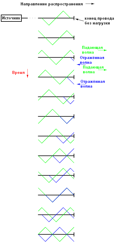
If we add these two signals, we will see that the third, stationary signal, is created along the entire length of the line: the red line in the figure below is the sum of the incident and reflected waves:

This third wave is the sum of the incident and reflected waves. It does not spread over the cable, as a falling or reflected wave. Pay attention to the points along the line where the incident and reflected waves always quench each other: these points never change position.

Standing waves are common in the physical world. Consider a rope tied at one end and shake it:

Knots (with points where there is no vibration) and antinodes (maximum vibration points) remain unchanged along the entire length of the rope. String instruments also create a standing wave, with nodes of maximum and minimum vibration along their length. The main difference between a string and a string instrument is that the instrument is already tuned to the correct vibration frequency:

Wind blowing through open pipes also produces standing waves. In this case, the air molecules in the pipe oscillate, not the solid body. A standing wave can end at a node (minimum amplitude) or at an antinode (maximum amplitude), and this depends on whether the other end of the tube is open or closed:


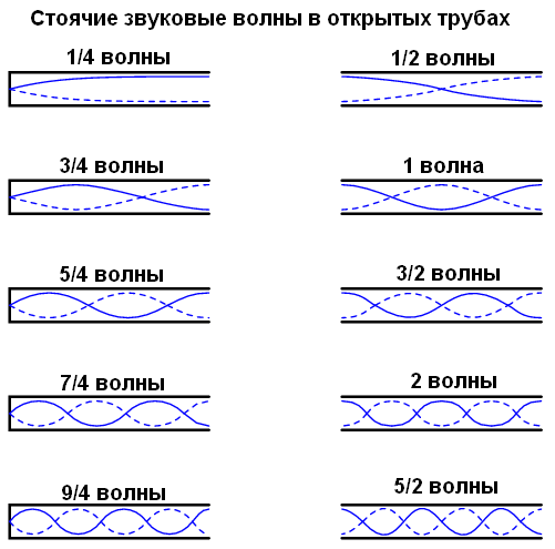
The closed end of the tube creates a knot, and the open end creates an antinode. By analogy, the string anchor is a knot, and the free end (if any) is an antinode.

Please note that inside the tube there may be standing waves of different frequencies. There are several resonant frequencies for any system that supports standing waves.

Higher frequencies must be a multiple of the base frequency.

The actual frequencies for any of these harmonics (overtones) depend on the physical size of the pipe and the speed of wave propagation (in this case, the speed of sound propagation).

In communication lines it is also possible to create standing waves, and their frequency will depend on the type of load at the end of the line, on the speed of propagation and physical length. The resonance in the transmission lines is more complicated than the resonance of the strings or air in the pipes, because we have to take into account the voltage and current of the waves.

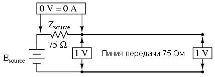
Resonance in transmission lines is easier to understand using computer simulations. To begin with, consider the agreed 75 ohm line:

Using SPICE to simulate a circuit, we specify a wave resistance of 75 Ohms (z0 = 75) and a propagation delay of 1 µs for the T1 line. This is a convenient way to express the physical length of a transmission line — the amount of time it takes to propagate a signal. For a real RG-59B / U cable, this will be 198 meters long. 1 μs corresponds to the frequency of 1 MHz. I will select frequencies from zero to this frequency to show how the system responds to different frequencies.
Here is the SPICE model:

Transmission line v1 1 0 ac 1 sin rsource 1 2 75 t1 2 0 3 0 z0 = 75 td = 1u rload 3 0 75 .ac lin 101 1m 1meg * Using "Nutmeg" program to plot analysis .end

Perform this simulation and build a graph of the voltage drop across the source resistance (Zsource) - this will be the current indicator and the voltage graph at the end of the line (voltage across the load). We will see that the voltage source is shown on the graph as vm (1) (the voltage between node 1 and ground point 0) is exactly 1 volt. The voltages at point 2 and 3 will be 0.5 volts. The voltage across the resistor - as a current indicator - will be 0.5 volts:


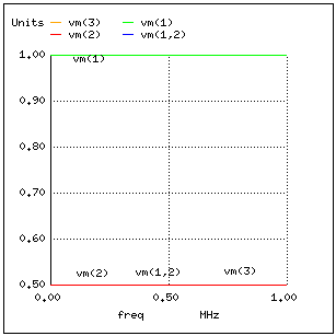
In a system where all resistances are perfectly matched, there can be no standing waves, and there are no resonances in the Bode graph .
Now let's change the resistance to 999 MΩ to simulate an open transmission line. We should definitely get reflected waves at some frequencies, from 1 MHz to 1 MHz:

Transmission line v1 1 0 ac 1 sin rsource 1 2 75 t1 2 0 3 0 z0 = 75 td = 1u rload 3 0 999meg .ac lin 101 1m 1meg * Using "Nutmeg" program to plot analysis .end

Here, the supply voltage of the vm (1) line and the voltage at the load remain at the same level - 1V. Other voltage drops are frequency dependent (also from 1 MHz to 1 MHz). There are five remarkable frequencies along the horizontal line: 0Hz, 250kHz, 500kHz, 750kHz, 1MHz. We study each point taking into account the voltage and current at various points in the circuit.

• 0 Hz (actually 1 MHz) - the signal is almost constant current, and the circuit behaves the same way as if 1 Volt DC was applied. The current does not flow, as indicated by the zero voltage drop across the Zsource resistor, the graph of vm (1,2), and the voltage on the source is equal to the voltage at the end of the line vm (2) (the voltage between point 2 and point 0).


• At 250 kHz, we see zero voltage at point 2, the maximum current from the source and the total voltage at the end of the line.


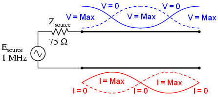
You may be wondering how this can be? How can we get the full voltage at the open end of the line if the input voltage is zero? The answer can be found in the paradox of the standing wave. At a frequency of 250 kHz, the line length is exactly of the wavelength. Since the end of the line is open, there can be no current, but the voltage will be. Thus, at the end of the wire there will be a node for the current (current is zero) and an antinode for voltage (maximum amplitude):


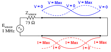
• At a frequency of 500 kHz, exactly half of the wave fits into the line, and here we see another point where the current is zero and the voltage again has a full amplitude:


• At 750 kHz, the picture is similar to the frequency of 250 kHz: the voltage at the source is zero, and the maximum current. ¾ waves fit into lines, as a result of which the source sees a short circuit at the point of connection to the transmission line, even though the other end of the line is open:


• When the frequency reaches 1 MHz, one full wave period fits into the line. At the moment, both the current and the voltage at the beginning of the line are equal to those at the end of the line. And if at the end of the line the current is zero (resistance is 999 MΩ), then the current at the beginning of the line is also zero. The voltage at the source is equal to the voltage at the load. In fact, the source sees an open circuit.


Similarly, a short circuit at the end of the line generates standing waves, although the nodes and antinodes in current and voltage change places: At the short-circuited end of the line there will be no voltage (node), but there will be a maximum current (antinode). Next comes SPICE modeling and an illustration of what happens at all interesting frequencies: 0Hz, 250 kHz, 500kHz, 750kHz, 1 MHz. A short circuit is simulated by a load resistance of 0 µOhm.

Transmission line v1 1 0 ac 1 sin rsource 1 2 75 t1 2 0 3 0 z0 = 75 td = 1u rload 3 0 1u .ac lin 101 1m 1meg * Using "Nutmeg" program to plot analysis .end

In both examples (open and short-circuited line) all energy is reflected. 100 percent of the incident wave reaches the end of the line and is reflected back to the source. If, however, the transmission line is loaded with some kind of resistance, there will be a difference between the maximum and minimum values ​​of voltage and current along the line.

Suppose we loaded the line with a resistor of 100 Ohm instead of 75:


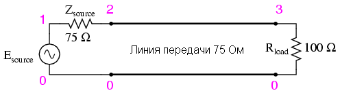
Let's build a model for this case:

Transmission line v1 1 0 ac 1 sin rsource 1 2 75 t1 2 0 3 0 z0 = 75 td = 1u rload 3 0 100 .ac lin 101 1m 1meg * Using "Nutmeg" program to plot analysis .end

If we run another SPICE analysis with the output of text values ​​instead of the graph, we may find that all interesting frequencies remain the same (DC, 250 kHz, 500 kHz, 750 kHz, and 1 MHz):

Transmission line v1 1 0 ac 1 sin rsource 1 2 75 t1 2 0 3 0 z0 = 75 td = 1u rload 3 0 100 .ac lin 5 1m 1meg .print ac v (1,2) v (1) v (2) v (3) .end

freq	v (1,2)	v (1)	v (2)	v (3)
1.000E-03	4.286E-01	1.000E + 00	5.714E-01	5.714E-01
2.500E + 05	5.714E-01	1.000E + 00	4.286E-01	5.714E-01
5.000E + 05	4.286E-01	1.000E + 00	5.714E-01	5.714E-01
7.500E + 05	5.714E-01	1.000E + 00	4.286E-01	5.714E-01
1.000E + 06	4.286E-01	1.000E + 00	5.714E-01	5.714E-01

At all frequencies, the voltage at the source at point 1 is 1 Volt, as it should be. The voltage at the load also remains constant, but has a smaller amplitude (0.5714 Volts). However, the line supply voltage (point 2, graph v (2)) and current (graph v (1.2)) indicates that the current from the source varies with frequency.






At the odd harmonics of the fundamental frequency (250 kHz and 750 kHz), we see different voltage levels at the beginning and end of the line, since at these frequencies standing waves create a node on one side of the line and antinodes on the other. In contrast to the open and short-circuited lines, the maximum values ​​do not reach either zero or 100% of the original signal. But we still have points with a minimum and maximum voltage. The same is true for current. If the load resistance of the line does not correspond to the line resistance of the line, we will have points of maximum and minimum current at some fixed points of the transmission line, corresponding to nodes and antinodes.

One way of expressing the level of standing waves is the ratio of the maximum amplitude (at the antinode point) to the minimum amplitude for voltage or current. This ratio is called KSV - standing wave ratio. If the line is open or short circuit, then the CWS equals infinity, since the minimum amplitude will be zero. In the example, a 75 Ω line with a load of 100 Ω CWS will be equal to 1.333: the maximum line voltage at 250 or 750 kHz (0.5714 V) divided by the minimum line voltage (0.4286 V).

The CWS can also be calculated, knowing the load resistance and the wave resistance of the line, dividing the larger value by the smaller one. In our example, 100Ω / 75Ω = 1,333.



A line with a perfectly matched load will have a CWS of 1. This is considered ideal not only because the reflected waves are energy that has not reached the load, but because of high voltage and current values: high voltage can create a breakdown in the insulation, but high current damage conductors.

Also, a line with a bad CWS acts as an antenna. This is undesirable: such an antenna can interfere with nearby wires. Interestingly, antennas are open transmission lines, and they work at CWS as close as possible to 1. This means that all energy is radiated.

The following photo shows the junction point in the radio link. Large copper pipes with a ceramic insulator are a rigid coaxial line with an impedance of 50 Ohms.



Flexible coaxial cable with a wave resistance of 50 Ohms. A white plastic pipe connects the gas inside the pipes: they are sealed to protect against moisture. Pay attention to the flat wires to connect the lines. Why are they not round? This is due to the skin effect, which makes a large cross-sectional area at high frequencies useless.

Like many communication lines, they operate at low CWS. As we will see in the next section, the phenomenon of standing waves in communication lines is not always harmful, as they can be used for a useful function: impedance conversion.

Impedance conversion

Standing waves at the resonant points of short-circuited or open lines can produce unusual effects. With a line length of ½ wavelength (and a factor of several times longer), the source sees the load as it is. The following illustrations show this:




In both cases, at the ends of the line there is an antinode for voltage and a node for current. The line simulates the load - infinite resistance, the source sees a break.
The same is true if there is a short circuit on the line: at the source connection point there will be a minimum of voltage and a maximum of current.




However, if the length of the line is equal to a quarter of the wavelength, the source at short circuit at the end of the line will see an open circuit, and the broken line will see it short-circuited.

The line is open, and the source sees a short circuit:




The line is closed, and the source sees a break:



At these frequencies, the transmission line behaves like a resistance transformer, turning the infinite resistance into zero and vice versa. This happens only at resonant points, when a quarter of a wave is placed in a line and is a multiple of more (3/4, 5/4, 7/4, 9/4 ...), but if the frequency is known and unchanged, then this phenomenon can be used for matching different wave resistances with each other.
Take for example the 75Ω transmission line with a 100Ω load. From the SPICE numerical simulation, we determine what resistance the source sees:






A simple equation relates the line impedance (Z0), load impedance (Zload) and input impedance (Zinput) for the unmatched line to the odd harmonic:


Consider a practical example when it is necessary to match the load 300Ω and the source 75Ω. All we have to do is calculate the correct line impedance and length for a quarter of the wavelength at 50 MHz.
First, calculate the line resistance. Z0 = Sqrt (75 * 300) = 150Ω.

Secondly, it is necessary to calculate the length of the line. Suppose the shortening coefficient is 0.85, the speed of light is 300 thousand km / s, the signal speed is 255 thousand km / s. We divide this speed by the frequency of the signal and get a wavelength of 5.1 meters. We need a quarter wavelength - it will be 1,275m.

Here is a diagram for SPICE analysis:



We can specify the length of the line by the signal delay. At a frequency of 50 MHz, the period will be 20 ns. The delay time for a quarter wavelength will be 5 ns.

Transmission line v1 1 0 ac 1 sin rsource 1 2 75 t1 2 0 3 0 z0 = 150 td = 5n rload 3 0 300 .ac lin 1 50meg 50meg .print ac v (1,2) v (1) v (2) v (3) .end

freq	v (1,2)	v (1)	v (2)	v (3)
5.000E + 07	5.000E-01	1.000E + 00	5.000E-01	1.000E + 00

At a frequency of 50 MHz at point 1-2, exactly half of it drops - 0.5 V, and the second half of the voltage falls on the communication line in the 2-0 circuit. This means that the source sees a load of 75Ω. The load, however, does not receive half, but 1 Volt (voltage v (3)). At a resistance of 75Ω, it drops 0.5V or 3.333mW - the same as at a load of 300 Ohms at a voltage of 1V. In accordance with the maximum power theorem (the Jacobi theorem), the maximum possible power is dissipated at the load. A quarter-wavelength transmission line, a wave impedance of 150Ω and a load of 300Ω behaves like a 75Ω load.

Of course, all this will work only at 50 MHz and odd harmonics. For other frequencies, the transmission line will have to be lengthened or shortened.

Oddly enough, the line of the same length will match the 300Ω source and 75Ω load. This shows that the phenomenon of impedance conversion is fundamentally different from the principle of operation of a two-winding transformer.

Transmission line v1 1 0 ac 1 sin rsource 1 2 300 t1 2 0 3 0 z0 = 150 td = 5n rload 3 0 75 .ac lin 1 50meg 50meg .print ac v (1,2) v (1) v (2) v (3) .end

freq	v (1,2)	v (1)	v (2)	v (3)
5.000E + 07	5.000E-01	1.000E + 00	5.000E-01	2.500E-01

In this case, the internal resistance of the source will drop 0.5V, or 833mW. The load will be 0.25V - the same 833mW.

This method is often used to match transmission lines and antennas in radio transmissions, since the frequency there is often known and unchanged. The minimum length of an impedance transducer is ¼ wavelength.