Practice using Freefem ++
In a previously published post, we talked about the use of the open source libraries Freefem ++ and NetGen in an aerodynamic process modeling program. In this article we will take a closer look at the basic features of Freefem ++ as a small introduction to its input language. This will give the initial information that developers often need when selecting third-party components for inclusion in the designed application.
Freefem ++ is a program designed to solve mathematical problems based on the finite element method. Freefem ++ can be used in both Windows and Linux environments. Official site www.freefem.org/ff++ . In our case, the Freefem ++ version 3.18.-1 was used. In the archive package, downloaded from the official site, there are three boot modules, the purpose of which is the following:
To run FreeFem ++ in the background as part of another program from the archive, the following files are required besides the boot module: libff.dll, libgcc_s_dw2-1.dll, libgfortran-3.dll, libgoto2.dll, libstdc ++ - 6.dll.
When launching the Freefem ++ boot module, the name of the script file written in a special C-like programming language is transferred to the command line. Using output statements or special save functions in the script, the results can be written to a file for further use.
Earlier, we showed that Freefem ++ can be used to form an STL description of a three-dimensional model consisting of elements with flat edges. To solve this problem it is necessary to perform a triangulation of faces. Consider how this is done using Freefem ++. Suppose you want to perform a triangulation of the surface defined by the boundaries (see. Fig. 1).

Fig. 1. Regions of the surface
')
Borders of areas for which it is necessary to execute a triangulation, are set in Freefem ++ in a parametric look. Consider the following code:
Freefem ++ defines scalar variable types: int, real, string, bool. A variable declaration is performed as in C ++, and the variable can be initialized, as is done for variable n.
Borders are defined by fragments using parameterized lines. The type of border is intended for this. Fragments of borders can only intersect at the ends. The declaration of a boundary fragment includes the boundary identifier, the parameter change boundary (in this case, the parameter t), and expressions for changing the x and y coordinates depending on the parameter. In the example, all fragments are segments.
The last statement in the considered code is plot, it is intended for graphical display of data of certain types. In this case, it displays a border consisting of fragments of borders. Fragments of the border are combined into a common border using the + operator. For each fragment, the parameter specifies the number of parts into which the fragment should be divided. This parameter will be reviewed again in a different context. The result of the execution of the specified plot operator is shown in Fig. 2
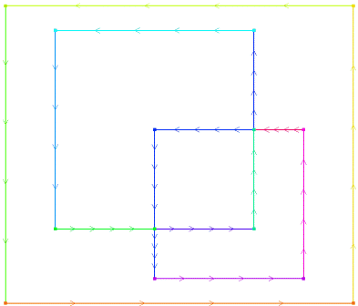
Fig. 2. The boundaries of the surface regions displayed by the plot operator
Now add the code that performs triangulation. In fig. 3 shows the result of its implementation.
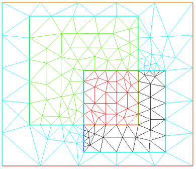
Fig. 3. Triangulation result
This code introduces the mesh variable Th. The mesh type is a software model of a triangulation mesh. To obtain an object of this type, in this case, the function buildmesh is used, by which the boundary of the split areas is passed to the input. The buildmesh functions can be passed an optional fixeborder parameter, the use of which ensures that the points on the line will not be changed during the triangulation process. The second operator, plot, in this case takes an object of the mesh type at the input and displays the grid of elements in the graphics window (Fig. 3).
As already shown, the border is represented as the sum of border fragments of the type border. The parameter specified for each fragment here has a dual purpose. Firstly, it indicates how many parts the fragment of the boundary for grid building is divided. Each part of the border fragment will become the side of the triangle of the formed grid. Secondly, the sign of the parameter indicates the area that should undergo triangulation. If the parameter is positive, then triangulation is performed to the left of the border fragment. If it is negative, then triangulation is performed to the right of the border. Let us explain this with an example. If in the above code the boundary was defined as: b0 (n) + b1 (n) + b2 (n) + b3 (n) + b4 (n) + b5 (-2) + b6 (n) + b7 (n) + b8 (n) + b9 (-2) + b10 (n) + b11 (n) + b12 (n) + b13 (-2) + b14 (-2) + b15 (n), where for b5, b9, b13 and b14 are divided into two segments with a negative value, then the triangulation would be performed as shown in Fig. four.
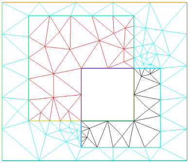
Fig. 4. Triangulation with an empty subregion
Add a code showing operations with a variable of type mesh, a loop operator and output to a file.
To output data to a file, the type ofstream is provided, an analogue of the file output stream from the fstream library for C ++. When initializing a file variable, you must specify the file name. If you only need to add data to the file, you need to specify the second initialization parameter append. You can perform a series of operations with a file variable. In the example, the precision function is used to set the number of digits after the decimal separator. There are several other functions that control the output format, similar to the manipulators from the iostream library. The << operator allows you to output the values of scalar types to the file. In the character string, you can use the end-of-line character '\ n', or for this purpose, output the global variable endl.
In the above code, there is a for statement that completely repeats the logic of the for statement in C ++. The increment and decrement operators also repeat similar C ++ operators.
Freefem ++ provides access to various mesh properties represented by the mesh type. We also note here that Freefem ++ provides the same interfaces for working with a two-dimensional mesh of the mesh type, and with a three-dimensional mesh of the mesh3 type. Therefore, here we consider this interface for the two types indicated, in order not to repeat its description for mesh3 later. As you can see from the example, the nt property returns the number of mesh elements (triangles for mesh or tetrahedrons for mesh3). You can also get the number of grid points — the nv property, the number of boundary elements — nbe.
Two types of indexing can be applied to an object of type mesh or mesh3: indexing with square brackets "[]" and indexing with parentheses "()". The first of them gives a mesh element (a triangle for a mesh or a tetrahedron for a mesh3) with a given index. Thus, Th [i] is a grid element (a triangle in this example) to which, in turn, certain functions provided for the element are applied. "()" - the index provides a vertex with a given index. To the top, operations of obtaining its coordinates can be applied. The following functions are applied to the grid element: indexing to obtain the vertices of the element, obtaining the label.
Freefem ++ defines the mesh3 type for a 3D mesh. Such a grid can be obtained using generation functions. For example, the buildlayers () function allows you to form a 3D grid by extruding 2D triangulation along the Z axis. However, Freefem ++ does not have its own generator. For these purposes, a third-party TetGen generator (official site wias-berlin.de/software/tetgen ) is used, and the corresponding functions of Freefem ++ are the program interface to this generator. TetGen cannot be used in commercial projects without the permission of the author. But if such a license creates a problem, then you can use another grid generator. Freefem ++ has the ability to import a 3D mesh from a file that matches the mesh format. A mesh file has the following format:
The mesh file is imported using the readmesh3 function, which specifies the file name:
To import a mesh from a mesh file, the order of the numbers of vertices of tetrahedra turns out to be critical. In the Freefem ++ source code, you can find a DataTet structure in the Mesh3dn.hpp file, which has a mesure () method for calculating the volume of the tetrahedron. If the vertices of the tetrahedron in the mesh file are followed in such a way that the calculated volume turns out to be negative, then Freefem ++ ends with an error. Therefore, the vertices in the mesh file must be listed so that this situation does not occur.
If necessary, the grid can be displayed in the graphic window with the function plot (see Fig. 5).
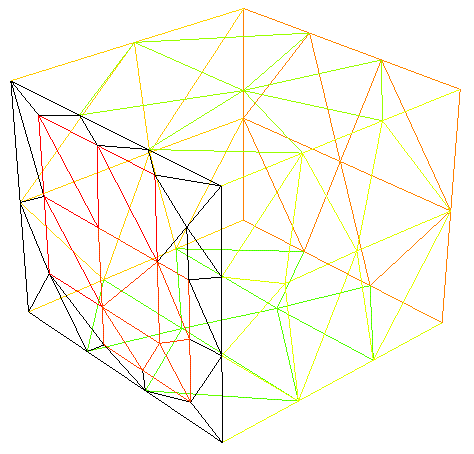
Fig. 5. 3D grid display by plot function
The main purpose of Freefem ++ is to solve systems of partial differential equations by the finite element method. For this, the functions involved in the system of equations are determined on a grid of finite elements. Freefem ++ allows you to determine the type of FE-space (finite element space). In accordance with the type of space, objects of functions of a certain space are introduced. For example,
where Vh is the type of space on the grid Th, f is a function on this space.
When declaring a finite element space type, the basis for the elements is indicated. It can take the values P03d - piecewise constant, P13d - piecewise linear, P23d - piecewise quadratic, etc. In fig. 6 shows the function from the example with a quadratic basis, and fig. 7 - the same function with a linear basis and with noticeable distortions.
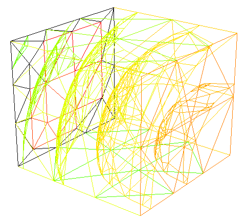
Fig. 6. A finite-element function with a quadratic basis
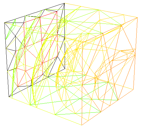
Fig. 7. Finite element function with linear basis.
To solve a system of partial differential equations in Freefem ++, a variational statement of the problem is specified, and the desired functions are formed when solving the problem. Based on the following script, we will look at how the variation language and other programming elements are written.
This example shows the following constructs. Finite element space can be defined for a vector field. In the example, the space VVh is defined for a vector field with four components, and Vh for a scalar field.
Freefem ++ provides the ability to declare macros that start with the macro keyword. In a macro substitution, the macro name will be replaced with the macro body, replacing the formal parameters with the actual ones. In the example there are two macros: Grad (u) and div (u1, u2, u3). In these macros, special notation dx, du, dz is used, which designate the differentials in the corresponding coordinates.
The function is declared using the func keyword. Moreover, if the function arguments are denoted by x, y, z, which are reserved words, then it is not necessary to specify the formal parameters.
The solve construct is used to record the variational formulation and solution of the problem. After the task name, unknown and test functions are listed. In this case, the Prob problem has two vector functions defined on the space VVh: [u1, u2, u3, p] is the desired and [v1, v2, v3, q] is a trial. After the equal sign, the expression for the variation formulation is written. In the example in this place there are two specific Freefem ++ constructs. To record the three-dimensional integral, a special int3d construction is used, in which the integration space is specified, in this case, it is the grid Th. In addition, the matrix transposition operator, denoted by an apostrophe, is used here. At the end of the variational formulation, the boundary conditions are written in the solve construction. The boundary condition is denoted by the special word on, after which the corresponding area in the object of the class of mesh3 is indicated in parentheses. Writing these labels to a mesh file was discussed above. For a region, the components of the desired field are listed and a constraint is written for each of them. The constraint can be an arbitrary expression. In the example, numbers and the function fup are set as a constraint.
When displaying the field component using the plot function, in the graphics window, a finite element space with isosurfaces is shown, as shown in Fig. 8. The number of isosurfaces can be set with the nbiso parameter in the script, and then manually changed in the graphics window.

Fig. 8. Result of the decision
Freefem ++ is a powerful tool for solving mathematical problems that can be used when developing applications, including commercial ones. In the latter case, a useful feature of Freefem ++ is the ability to import a 3D finite element mesh, which allows the use of third-party grid generators.
Getting and running Freefem ++
Freefem ++ is a program designed to solve mathematical problems based on the finite element method. Freefem ++ can be used in both Windows and Linux environments. Official site www.freefem.org/ff++ . In our case, the Freefem ++ version 3.18.-1 was used. In the archive package, downloaded from the official site, there are three boot modules, the purpose of which is the following:
- FreeFem ++. Exe is a full-fledged version of the program, which, if necessary, displays a graphical window with the results of the solution. If necessary, you can specify two keys during the call: -nowait to ensure that Freefem ++ is completed without confirmation of completion by the user, and -nw - to refuse to display the graphic window with the results of the decision.
- FreeFem ++ - mpi.exe - for paralleling calculations based on MPI.
- FreeFem ++ - nw.exe - to call from applications, ignores graphical output of results. In order that he also did not expect confirmation of completion of work with the program, it is necessary to specify the –nowait key in the command line.
To run FreeFem ++ in the background as part of another program from the archive, the following files are required besides the boot module: libff.dll, libgcc_s_dw2-1.dll, libgfortran-3.dll, libgoto2.dll, libstdc ++ - 6.dll.
When launching the Freefem ++ boot module, the name of the script file written in a special C-like programming language is transferred to the command line. Using output statements or special save functions in the script, the results can be written to a file for further use.
2D triangulation
Earlier, we showed that Freefem ++ can be used to form an STL description of a three-dimensional model consisting of elements with flat edges. To solve this problem it is necessary to perform a triangulation of faces. Consider how this is done using Freefem ++. Suppose you want to perform a triangulation of the surface defined by the boundaries (see. Fig. 1).
Fig. 1. Regions of the surface
')
Borders of areas for which it is necessary to execute a triangulation, are set in Freefem ++ in a parametric look. Consider the following code:
  int n = 5;

 border b0 (t = 0,1) {x = 7 * t;  y = 0;  }
 border b1 (t = 0,1) {x = 7;  y = 0 + 6 * t;  }
 border b2 (t = 0,1) {x = 7 - 7 * t;  y = 6;  }
 border b3 (t = 0,1) {x = 0;  y = 6 - 6 * t;  }
 border b4 (t = 0,1) {x = 1 + 2 * t;  y = 1.5;  }
 border b5 (t = 0,1) {x = 5;  y = 1.5 + 2 * t;  }
 border b6 (t = 0,1) {x = 5 - 4 * t;  y = 5.5;  }
 border b7 (t = 0,1) {x = 1;  y = 5.5 - 4 * t;  }
 border b8 (t = 0,1) {x = 5;  y = 3.5 + 2 * t;  }
 border b9 (t = 0,1) {x = 3 + 2 * t;  y = 1.5;  }
 border b10 (t = 0,1) {x = 3 + 3 * t;  y = 0.5;  }
 border b11 (t = 0,1) {x = 6;  y = 0.5 + 3 * t;  }
 border b12 (t = 0,1) {x = 6 - 1 * t;  y = 3.5;  }
 border b13 (t = 0,1) {x = 3;  y = 3.5 - 2 * t;  }
 border b14 (t = 0,1) {x = 5 - 2 * t;  y = 3.5;  }
 border b15 (t = 0,1) {x = 3;  y = 1.5 - 1 * t;  }

 plot (b0 (n) + b1 (n) + b2 (n) + b3 (n) + b4 (n) + b5 (n) + b6 (n) + b7 (n) + b8 (n) + b9 (n ) + b10 (n)
  + b11 (n) + b12 (n) + b13 (n) + b14 (n) + b15 (n));
Freefem ++ defines scalar variable types: int, real, string, bool. A variable declaration is performed as in C ++, and the variable can be initialized, as is done for variable n.
Borders are defined by fragments using parameterized lines. The type of border is intended for this. Fragments of borders can only intersect at the ends. The declaration of a boundary fragment includes the boundary identifier, the parameter change boundary (in this case, the parameter t), and expressions for changing the x and y coordinates depending on the parameter. In the example, all fragments are segments.
The last statement in the considered code is plot, it is intended for graphical display of data of certain types. In this case, it displays a border consisting of fragments of borders. Fragments of the border are combined into a common border using the + operator. For each fragment, the parameter specifies the number of parts into which the fragment should be divided. This parameter will be reviewed again in a different context. The result of the execution of the specified plot operator is shown in Fig. 2
Fig. 2. The boundaries of the surface regions displayed by the plot operator
Now add the code that performs triangulation. In fig. 3 shows the result of its implementation.
 mesh Th = buildmesh (b0 (n) + b1 (n) + b2 (n) + b3 (n) + b4 (n) + b5 (n) + b6 (n) + b7 (n) + b8 (n) + b9 (n) + b10 (n)
  + b11 (n) + b12 (n) + b13 (n) + b14 (n) + b15 (n), fixeborder = 1);
 plot (Th);
Fig. 3. Triangulation result
This code introduces the mesh variable Th. The mesh type is a software model of a triangulation mesh. To obtain an object of this type, in this case, the function buildmesh is used, by which the boundary of the split areas is passed to the input. The buildmesh functions can be passed an optional fixeborder parameter, the use of which ensures that the points on the line will not be changed during the triangulation process. The second operator, plot, in this case takes an object of the mesh type at the input and displays the grid of elements in the graphics window (Fig. 3).
As already shown, the border is represented as the sum of border fragments of the type border. The parameter specified for each fragment here has a dual purpose. Firstly, it indicates how many parts the fragment of the boundary for grid building is divided. Each part of the border fragment will become the side of the triangle of the formed grid. Secondly, the sign of the parameter indicates the area that should undergo triangulation. If the parameter is positive, then triangulation is performed to the left of the border fragment. If it is negative, then triangulation is performed to the right of the border. Let us explain this with an example. If in the above code the boundary was defined as: b0 (n) + b1 (n) + b2 (n) + b3 (n) + b4 (n) + b5 (-2) + b6 (n) + b7 (n) + b8 (n) + b9 (-2) + b10 (n) + b11 (n) + b12 (n) + b13 (-2) + b14 (-2) + b15 (n), where for b5, b9, b13 and b14 are divided into two segments with a negative value, then the triangulation would be performed as shown in Fig. four.
Fig. 4. Triangulation with an empty subregion
Add a code showing operations with a variable of type mesh, a loop operator and output to a file.
 ofstream fout ("triangulation.out");
 fout.precision (14);

 fout << Th.nt << endl;
 for (int i = 0; i <Th.nt; i ++)
 {
   fout
     << Th [i] [0] .x << ""
     << Th [i] [0] .y << ""
     << Th [i] [1] .x << ""
     << Th [i] [1] .y << ""
     << Th [i] [2] .x << ""
     << Th [i] [2] .y << ""
     << endl;
 }
To output data to a file, the type ofstream is provided, an analogue of the file output stream from the fstream library for C ++. When initializing a file variable, you must specify the file name. If you only need to add data to the file, you need to specify the second initialization parameter append. You can perform a series of operations with a file variable. In the example, the precision function is used to set the number of digits after the decimal separator. There are several other functions that control the output format, similar to the manipulators from the iostream library. The << operator allows you to output the values of scalar types to the file. In the character string, you can use the end-of-line character '\ n', or for this purpose, output the global variable endl.
In the above code, there is a for statement that completely repeats the logic of the for statement in C ++. The increment and decrement operators also repeat similar C ++ operators.
Freefem ++ provides access to various mesh properties represented by the mesh type. We also note here that Freefem ++ provides the same interfaces for working with a two-dimensional mesh of the mesh type, and with a three-dimensional mesh of the mesh3 type. Therefore, here we consider this interface for the two types indicated, in order not to repeat its description for mesh3 later. As you can see from the example, the nt property returns the number of mesh elements (triangles for mesh or tetrahedrons for mesh3). You can also get the number of grid points — the nv property, the number of boundary elements — nbe.
Two types of indexing can be applied to an object of type mesh or mesh3: indexing with square brackets "[]" and indexing with parentheses "()". The first of them gives a mesh element (a triangle for a mesh or a tetrahedron for a mesh3) with a given index. Thus, Th [i] is a grid element (a triangle in this example) to which, in turn, certain functions provided for the element are applied. "()" - the index provides a vertex with a given index. To the top, operations of obtaining its coordinates can be applied. The following functions are applied to the grid element: indexing to obtain the vertices of the element, obtaining the label.
3D mesh
Freefem ++ defines the mesh3 type for a 3D mesh. Such a grid can be obtained using generation functions. For example, the buildlayers () function allows you to form a 3D grid by extruding 2D triangulation along the Z axis. However, Freefem ++ does not have its own generator. For these purposes, a third-party TetGen generator (official site wias-berlin.de/software/tetgen ) is used, and the corresponding functions of Freefem ++ are the program interface to this generator. TetGen cannot be used in commercial projects without the permission of the author. But if such a license creates a problem, then you can use another grid generator. Freefem ++ has the ability to import a 3D mesh from a file that matches the mesh format. A mesh file has the following format:
- At the beginning of the file, the format version information (MeshVersionFormatted 1), the dimension of the space (Dimension 3) are recorded.
 MeshVersionFormatted 1
 Dimension 3
- After the Vertices keyword, the number of vertices of the grid is indicated and the vertices are listed, for which the X, Y, Z coordinates and the vertex label are indicated.
 Vertices
 65
 7 5 1.5 0
 7 3 1.5 0
 7 3 0.5 0
 7 5 3.5 0
 ...
- After the Tetrahedra keyword, the number of grid elements is indicated and the elements for which four vertex numbers and a label are recorded are listed.
 Tetrahedra
 185
 52 56 49 50 0
 3 18 14 61 0
 47 64 57 54 0
 ...
- After the Triangles keyword, the number of boundary triangles is recorded. For each triangle, the numbers of the vertices of the nodes of the grid that are the vertices of these triangles are listed, and the boundary mark is indicated.
 Triangles
 96
 2 3 8 2
 2 8 1 2
 4 1 7 2
 ...
- File ends with the End keyword
The mesh file is imported using the readmesh3 function, which specifies the file name:
 mesh3 Th;
 Th = readmesh3 ("example3d.mesh");
 plot (Th);
To import a mesh from a mesh file, the order of the numbers of vertices of tetrahedra turns out to be critical. In the Freefem ++ source code, you can find a DataTet structure in the Mesh3dn.hpp file, which has a mesure () method for calculating the volume of the tetrahedron. If the vertices of the tetrahedron in the mesh file are followed in such a way that the calculated volume turns out to be negative, then Freefem ++ ends with an error. Therefore, the vertices in the mesh file must be listed so that this situation does not occur.
If necessary, the grid can be displayed in the graphic window with the function plot (see Fig. 5).
Fig. 5. 3D grid display by plot function
Solution of systems of differential equations
The main purpose of Freefem ++ is to solve systems of partial differential equations by the finite element method. For this, the functions involved in the system of equations are determined on a grid of finite elements. Freefem ++ allows you to determine the type of FE-space (finite element space). In accordance with the type of space, objects of functions of a certain space are introduced. For example,
     fespace Vh (Th, P23d);
     Vh f = x ^ 2 + y ^ 2 + z ^ 2;
where Vh is the type of space on the grid Th, f is a function on this space.
When declaring a finite element space type, the basis for the elements is indicated. It can take the values P03d - piecewise constant, P13d - piecewise linear, P23d - piecewise quadratic, etc. In fig. 6 shows the function from the example with a quadratic basis, and fig. 7 - the same function with a linear basis and with noticeable distortions.
Fig. 6. A finite-element function with a quadratic basis
Fig. 7. Finite element function with linear basis.
To solve a system of partial differential equations in Freefem ++, a variational statement of the problem is specified, and the desired functions are formed when solving the problem. Based on the following script, we will look at how the variation language and other programming elements are written.
 mesh3 Th = readmesh3 ("example3d.mesh");

 fespace VVh (Th, [P2, P2, P2, P1]);
 fespace Vh (Th, P23d);

 macro Grad (u) [dx (u), dy (u), dz (u)] //
 macro div (u1, u2, u3) (dx (u1) + dy (u2) + dz (u3)) //

 VVh [u1, u2, u3, p];
 VVh [v1, v2, v3, q];

 func fup = (1-x) * (x) * y * (1-y) * 16;

 solve Prob ([u1, u2, u3, p], [v1, v2, v3, q]) =
   int3d (Th, qforder = 3) (Grad (u1) '* Grad (v1) + Grad (u2)' * Grad (v2) + Grad (u3) '* Grad (v3)
		        - div (u1, u2, u3) * q - div (v1, v2, v3) * p + 1e-10 * q * p)
 + on (5, u1 = 0, u2 = 0, u3 = 0)
 + on (1, u1 = fup, u2 = 0, u3 = 0);

 plot (p, nbiso = 10);
This example shows the following constructs. Finite element space can be defined for a vector field. In the example, the space VVh is defined for a vector field with four components, and Vh for a scalar field.
Freefem ++ provides the ability to declare macros that start with the macro keyword. In a macro substitution, the macro name will be replaced with the macro body, replacing the formal parameters with the actual ones. In the example there are two macros: Grad (u) and div (u1, u2, u3). In these macros, special notation dx, du, dz is used, which designate the differentials in the corresponding coordinates.
The function is declared using the func keyword. Moreover, if the function arguments are denoted by x, y, z, which are reserved words, then it is not necessary to specify the formal parameters.
The solve construct is used to record the variational formulation and solution of the problem. After the task name, unknown and test functions are listed. In this case, the Prob problem has two vector functions defined on the space VVh: [u1, u2, u3, p] is the desired and [v1, v2, v3, q] is a trial. After the equal sign, the expression for the variation formulation is written. In the example in this place there are two specific Freefem ++ constructs. To record the three-dimensional integral, a special int3d construction is used, in which the integration space is specified, in this case, it is the grid Th. In addition, the matrix transposition operator, denoted by an apostrophe, is used here. At the end of the variational formulation, the boundary conditions are written in the solve construction. The boundary condition is denoted by the special word on, after which the corresponding area in the object of the class of mesh3 is indicated in parentheses. Writing these labels to a mesh file was discussed above. For a region, the components of the desired field are listed and a constraint is written for each of them. The constraint can be an arbitrary expression. In the example, numbers and the function fup are set as a constraint.
When displaying the field component using the plot function, in the graphics window, a finite element space with isosurfaces is shown, as shown in Fig. 8. The number of isosurfaces can be set with the nbiso parameter in the script, and then manually changed in the graphics window.
Fig. 8. Result of the decision
findings
Freefem ++ is a powerful tool for solving mathematical problems that can be used when developing applications, including commercial ones. In the latter case, a useful feature of Freefem ++ is the ability to import a 3D finite element mesh, which allows the use of third-party grid generators.
Source: https://habr.com/ru/post/182396/
All Articles