How to run a program without an operating system: part 4. Parallel computing
After a long break, we continue to do interesting things, as always on a clean iron without an operating system. In this part of the article, we will learn how to use the full potential of processors: we will run the program on several processor cores in a completely parallel mode at once. To do this, we need to do a lot to extend the functionality of the program obtained in Part 3 .
Just because doing some calculations on the processor cores is boring, so we need a task that requires large computational resources, is well decomposed into parallel computing, and it looks cool. We propose to make a program that renders a simple 3D scene using the ray tracing algorithm, or, in a simple way, Ray Tracing .
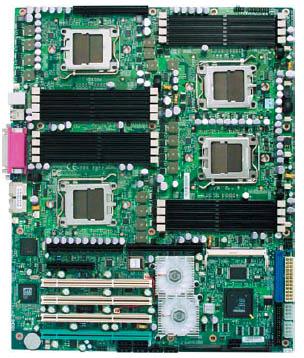
Let's start from the beginning: our goal is parallel computing on all processor cores. All modern processors for the PC, and the ARM already too (I am silent about the GPU) are multi-core processors. What does this mean? This means that instead of a single computing core, the processor on one computer has several cores. In general, everything looks somewhat more complicated: several sockets (processor chips) can be installed on a computer, several physical cores can be located within each chip (within one crystal), and several logical cores can be located within each physical core ( for example, those that arise when using technology Hyper Threading). All this is schematically represented in the figure below, and is called a topology.
')

Obviously, sockets are just several installed processors of the same motherboard. Below are some more pictures for clarity.
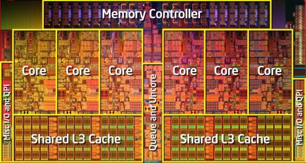
Among all this, the most interesting is the presence of logical cores . This is the principle of SMT (Simultaneous Multithreading), which means, in practice, the execution of successive instructions from another logical stream, during which parts of the processor were released, waiting for the end of the execution of instructions from the main thread. Each physical processor core consists of many components (cache, pipelines, ALU, FPU, ...), many parts operate independently of each other and need to be synchronized, so while the instruction waits for data from the cache or memory before the end of execution, why not execute others instructions from another thread using the same instructions? More information and pictures can be found on this link or in official documents of Intel, AMD, ARM.
In this article, the details of the topology will be important only to improve the optimization (and all the cores will be perceived as the same). You can get the topology programmatically using the CPUID instructions, but more on that next time.
Let's introduce some more concepts:
SMP (Symmetric Multiprocessing) - means the symmetric use of all processors; for example, all processor cores can access the same RAM in full, all processor cores are the same and behave the same.
AMP (Asymmetric Multiprocessing) as opposed to the previous concept, means that at least one core behaves differently than others. For example, the joint work of CPU and GPU can be considered as an example of AMP.
NUMA (Non-Uniform Memory Access) - non-uniform access of processors to different areas of memory. In fact, it means that each processor core can access the entire memory, but for each core there is a memory area to which it refers faster than the rest. Again used for optimization.
In modern computer has all of these principles and technologies.
We will consider the SMP in its purest form. When the system starts, the processor itself selects one arbitrary core and calls it the Boot Strap Processor (BSP), all others become the Application Processor (AP). BSP begins to execute the BIOS code, which, in turn, finds and starts all the processor cores in the system, performs their preliminary initialization and safely turns them off. Thus, our program after the start will work on one BSP core of the processor, so our goal looks, at first glance, quite simple: find out how many cores are on a computer, then run and configure each core in the system, and make all cores perform one computational task for the common good.
In order to achieve our goal you need to answer a few questions:
How to determine the number and topology of processors and cores in the system?
To do this, you need to use the wonderful ACPI interface, and to determine the topology, use the CPUID.
How to identify a specific processor core?
To do this, use an APIC device, or rather LAPIC, which each processor core in the system has, possesses a unique identifier for the system (such as the PID for processes), and is responsible for delivering interrupts to a specific processor core.
How to run one core from another core?
It is enough to send an interrupt from one processor core to another. This signal is called IPI (Inter Processor Interrupt). To send it, it is enough to use the LAPIC device on one of the cores, writing a certain value to its register.
How to stop the execution of the processor core?
It is enough to call the HLT instruction on this kernel.
Now a little more. ACPI (not to be confused with APIC ) - this is the Advanced Configuration and Power Interface - in fact it is a standard interface through which the operating system can obtain information about the computer, its detailed configuration, and control the power of the computer. This interface consists of a power management device (which is called an ACPI device, and, by the way, is present in PCI ( look at the article )), and several ACPI tables that are located in the computer’s RAM and contain information about the system. In addition to information about the processor cores on a computer, some ACPI tables store information even about the physical dimensions and form factor of the computer (for example, you can learn from them that the program runs on a tablet ...). There are a lot of tables, and their full description can be found here , and we are only interested in the MADP referenced by the RSDT, the pointer to which is in the RSDP table, which can be found somewhere in the vicinity of the BIOS. A simplified diagram of the main ACPI tables is presented as follows:
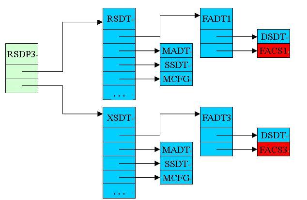
For now, all you need to know is that MADT contains records with information about the processor cores. Each entry contains the LAPIC identifier of this core (8 bits long, which means no more than 256 cores of any type in the system) and the Enable bit (which indicates whether this core can be used or reserved).
Now LAPIC is Local APIC, and APIC (not to be confused with ACPI ) is the Advanced Programmable Interrupt Controller, which replaces the old PIC (Programmable Interrupt Controller). PIC used to immediately deliver interrupts to the processor, and now it does it through LAPIC. Local APIC is not the only type of APIC - there is also IO APIC - which is a separate interrupt controller and is responsible for distributing interrupts between the processor cores on the system. Total picture is as follows:
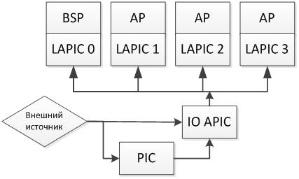
At first glance, it looks difficult, but if you look at it, then everything is quite reasonable: the PIC — an interrupt controller that has been used for a long time — has remained and has not gone anywhere, it is still part of the chipset on the motherboard. With the advent of multi-core IO APIC added, which now distributes interrupts from the PIC and other sources between the cores, because someone needs to do this. Each LAPIC is provided with a unique identifier that is used in IPI and IO APIC configuration. Also in the number LAPIC coded its topology. BSP always has a LAPIC ID of 0.
To program LAPIC, you need to read and write data to its registers (as with any other device), its registers are located in memory at 0xFEE00000. In fact, this address may be different, but you can always find it through a special MSR (Model Specific Register - these registers are read and written via the rdmsr / wrmsr instructions). For all cores, this address is often the same, but each core at this address has its own personal LAPIC. This device has many registers, but we need only one - ICR (Interrupt Control Register) which allows you to send IPI.
To start a processor core, this core needs to send as many as three IPIs that will force the other core to turn on: INIT IPI, then STARTUP IPI, and another STARTUP IPI. The second STARTUP IPI (or SIPI) is needed to complete the initialization process, since the first could be canceled, and the second will be ignored if the first SIPI is successful. Nothing can be done - such rules. To send each IPI, you simply need to write certain bytes to the ICR register of your LAPIC. These bytes will include the LAPIC identifier byte to which the IPI is sent, and the type of IPI to be sent. For SIPI, 2 more bytes will be used, from which the memory address from which the AP will be launched will be determined.
The latter is very convenient, since we will need to start the processor first from our code, which will transfer the processor to Protected Mode (yes, the processor after INIT-SIPI-SIPI runs in Real Mode, which does not suit us). The processor initialization code will be discussed in detail later. Yes, we won't do without a raw assembler.
You can read more about LAPIC and IO APIC in the Intel processor manual .
Now it remains to deal with several trifles: Lock , FPU and the Ray Tracing algorithm itself (payload).
The first thing we still need is the ability to synchronize the work of all the cores. To do this, you need to write the Lock code, which would expect to appear in the memory, for example, ones. How to make Lock correctly? The most obvious option is to write a simple while (1), which expects the appearance of a zero at a certain address, and immediately write down the unit at this address, while the other cores did not have time to do this. And to unlock the lock you need to write a zero.
Now FPU (Floating Point Unit) is a special module on the processor, which is used for arithmetic calculations with a floating point. In other words, if you want to use variables of type float and double in your program, then you need to initialize this module. In all modern operating systems, this makes the core of the operating system for you, but in our case it will be necessary. However, it is not difficult at all - just a couple of instructions in assembly language. We will need float because Ray Tracing will not work otherwise.
How do we do Ray Tracing ? This algorithm is beyond the scope of this article, so it will not be explained here, but there are many good articles about it . For our case, we just take the finished program and modify it a little.
Now that the theory is over, let's start writing the program.
! IMPORTANT !: All further actions can be successfully carried out only after successful completion of all 6 steps from the third part of the article “How to run a program without an operating system”
First of all, you need to slightly clear the existing code from unnecessary files and functions. We need a full-fledged mathematical library, so we need to delete the extra files from common: we delete the file common / s_floor.c .
We don’t need to draw a fractal - we need Ray Tracing, so you can delete fractal.c. But since the graphics mode is still needed, we write the following code in kernel.c:
1. add a few declarations in front of the main function, which, among other things, define the screen resolution and the image that will be rendered:
i
2. change the main function:
3. delete the line:
Now you can add a complete mathematical library. In fact, we only need the functions sqrt, tan and pow - they are used in the Ray Tracing algorithm.
1. create the fdlibm directory in the root .
2. in this directory, download the fdlibm library from here . You need to download all the files from this folder.
3. Now you need to replace the makefile with a simpler one (at the same time you can check the list of files). Compiling will use the same flags as the main makefile in the root. This will build a simple library fdlibm.a. Contents of the new makefile:
4. so that everything is going to make a change to k_standard.c . We need to declare errno and define an empty function fputs, which in our case has no meaning without a file system and a graphic display. To do this, replace the lines:
on the lines:
As usual, you need to slightly expand the definitions that will be used later in the program.
1. This time C ++ will be used, even with templates, therefore, to avoid a number of errors, you need to correct the include / string.h file. In it, you need to add an explicit type conversion in all places where void * is converted to char *. I got this line: 42, 53,54,79,80. Everywhere a similar change, for example, the corrected line 42 looks like this:
p = (char *) addr;
2. You need to add a few definitions for the math library. These include several global variable definitions, several types, several constants, and error codes that fdlibm uses. As a result, we add the following code to include / types.h (before the last #endif at the end of the file):
3. Add the file include / errno.h with the following code:
4. Now, you need to add a lot of definitions related to hardware, SMP setup, ACPI, LAPIC, and special processor register setup functions. To do this, create a file include / hardware.h, to which we add the following code . This time we placed two files with ready-made code on github. This is due to the fact that the code is relatively long (~ 500 lines), therefore, it is inconvenient to write it in the framework of the article. We emphasize that the code is supplied with a large number of comments in Russian, so the code on github can be considered a continuation of the article. In the paragraph we will give the contents of the file:
a. definitions of structures used to parse ACPI tables. This code is based on the official ACPI specification. The code contains only definitions for the tables we need (RSDP, RSDT, MADT).
b. The following file declares several inline functions containing assembler instructions. For the most part, the functions are very small, although they look cumbersome due to the peculiarities of using assembler in gcc, where a typical construction looks like this: __asm__ __volatile__ ("<instructions>": <output parameters>: <input parameters>); The code of these functions by name can be found on the Internet in different places, like in the code of FreeBSD, Linux, and such projects as Bitvisor. We also need the following functions: rdtsc, __rdmsr, __rdmsrl, __wrmsr, __wrmsrl, __rep_nop and __cpuid_count, __get_cr0, __set_cr0.
c. I especially want to highlight two functions that we called SmpSpinlock_LOCK and SmpSpinlock_UNLOCK. Both functions are taken from orangetide.com/src/bitvisor-1.3/include/core/spinlock.h and are also written in assembler. They are functions of working with a synchronization object for processor cores operating simultaneously. These are simple locks. The essence of their work is simple: as a lock, one byte is used in memory, which can take the value 0 or 1. If 0, then the lock is open, and if 1, then it is closed. The essence of the SmpSpinlock_LOCK function is to wait for the 0 value in the lock byte and set this byte to 1. The normal cycle is used for waiting using the “pause” instruction, which allows you to optimize the processor performance and reduce its power consumption during the wait cycles. To read and simultaneously set the value of 1 to the memory byte, the instruction “xchg” is used, which allows atomic exchange of values between the memory and the register. Atomicity means that another processor core will not be able to disrupt the operation of this instruction and will stick into the middle of its operation.
d. The hardware.h code contains a description of several constants associated with LAPIC. They are taken from the Intel documentation.
e. At the end of the file, another assembler function __enable_fpu is declared, which performs the inclusion of FPU on the processor. Recall that this is necessary for working with types of float. The function is the execution of two instructions: “fnclex” and “fninit”, which are necessary to enable FPU on the core.
Now, you can start creating the smp.c file, which will contain functions for working with several processor cores. The most important part of this file is assembler code that will be executed on newly launched kernels. The code smp.c is also located on github and is provided with a large number of comments with explanations; Part of the code had to be collected from a variety of sources on the Internet, and some had to be written by myself. The fact is that multi-core configuration is a specific case for each OS, so the code contains a lot of what a particular OS needs. The purpose of the author of the article was to simplify this code so that it was possible to demonstrate the essence of what is happening and the minimum of actions that must be performed to use SMP. The smp.c code contains two parts:
1. code to search and enable each AP. The beginning of the entire initialization occurs with the call to the SmpPrepare function. For the operation of some subfunctions, it is necessary to observe not a large time delay. Correctly, these delays should be done using a timer or CMOS, but for example, a delay is used based on waiting for a certain value of the TSC counter (processor clock counter that has passed since its start). The following steps are performed within SmpPrepare:
2. code running on each AP. This code starts with an assembler. It is located immediately at the beginning of the smp.c. file. In this assembly code, each line is commented. If we describe this assembly code briefly, it performs the following actions:
The function SmpApMain defines the index of the processor. The index is its number from 0 to N - where N-1 is the total number of cores on the computer. Then the counter of running cores increases synchronously, which is used to wait for all processors to start. Then the processor core goes into waiting for the launch of the payload flag. As soon as the flag is turned on, the ap_cpu_worker function is called — which performs the payload (Ray-Tracing).
The most difficult part behind. Now we need to add the payload in the form of the Ray Tracing algorithm. The algorithm itself is beyond the scope of this article, so theory and practice can be obtained from these resources . We will not comment the Ray Tracing code. Instead, we take the ready code as a basis and tell you how to change it in order to compile it in our program. We take the code from here as a basis. It will need to remove the dynamic allocation of memory and STL, replacing everything with a static array. Then, you need to fix the render function so that it can render only the area of the image in rows. Last, you will need to implement the ap_cpu_worker function, which calls render with certain parameters.
1. create a ray.cpp file. Copy the final code into it .
2. replace the lines in it:
On the lines:
3. delete the following lines:
and these:
4. replace:
On:
5. in the whole ray.cpp file , replace spheres.size () with spheres_size (only 3 replacements).
6. replace the render function in this way:
7. Accordingly, in the entire file, correct the two remaining calls to the trace function, adding another spheres_size parameter:
replaced by:
and this:
on:
8. at the end of the file, instead of the main function, we add the ray_main and ap_cpu_worker functions :
It remains only to modify the makefile so that everything compiles. To do this, we make the following changes:
1. update OBJFILES:
2. add a target for compiling C ++:
3. Next, you need to change the call line of the binder to connect the new library:
4. Now you need to build a library:
5. Now you can rebuild the project:
6. we start the project with an option of emulation of the 4th nuclear processor to be convinced that everything works:
If everything is done correctly, then we should see such beauty here:

As in the previous parts of the article, using the dd command, you can copy the hdd.img image to a USB flash drive and test the operation of the program on a real computer.
The result was an interesting program that uses all the cores of modern processors. This article opens up opportunities for developing programs that are sharpened by time-consuming calculations. It is important to note that, as in previous articles, there is no operating system; therefore, all calculations are performed using all available hardware resources. The program does not even handle interrupts - they are just turned off. Therefore, at what speed everything will be drawn and will determine the actual computational capabilities of your processor. Of course, this is all true if the program is running on bare metal. Our Intel i5 spends about 800 milliseconds to draw this picture. It will be interesting to see in the comments information about the speed that you got on real hardware.
Links to the following articles of the cycle:
" How to run a program without an operating system: part 5. Accessing the BIOS from the OS "
" How to run a program without an operating system: part 6. Support for working with disks with the FAT file system "
Just because doing some calculations on the processor cores is boring, so we need a task that requires large computational resources, is well decomposed into parallel computing, and it looks cool. We propose to make a program that renders a simple 3D scene using the ray tracing algorithm, or, in a simple way, Ray Tracing .
Let's start from the beginning: our goal is parallel computing on all processor cores. All modern processors for the PC, and the ARM already too (I am silent about the GPU) are multi-core processors. What does this mean? This means that instead of a single computing core, the processor on one computer has several cores. In general, everything looks somewhat more complicated: several sockets (processor chips) can be installed on a computer, several physical cores can be located within each chip (within one crystal), and several logical cores can be located within each physical core ( for example, those that arise when using technology Hyper Threading). All this is schematically represented in the figure below, and is called a topology.
')
Obviously, sockets are just several installed processors of the same motherboard. Below are some more pictures for clarity.
Among all this, the most interesting is the presence of logical cores . This is the principle of SMT (Simultaneous Multithreading), which means, in practice, the execution of successive instructions from another logical stream, during which parts of the processor were released, waiting for the end of the execution of instructions from the main thread. Each physical processor core consists of many components (cache, pipelines, ALU, FPU, ...), many parts operate independently of each other and need to be synchronized, so while the instruction waits for data from the cache or memory before the end of execution, why not execute others instructions from another thread using the same instructions? More information and pictures can be found on this link or in official documents of Intel, AMD, ARM.
In this article, the details of the topology will be important only to improve the optimization (and all the cores will be perceived as the same). You can get the topology programmatically using the CPUID instructions, but more on that next time.
Let's introduce some more concepts:
SMP (Symmetric Multiprocessing) - means the symmetric use of all processors; for example, all processor cores can access the same RAM in full, all processor cores are the same and behave the same.
AMP (Asymmetric Multiprocessing) as opposed to the previous concept, means that at least one core behaves differently than others. For example, the joint work of CPU and GPU can be considered as an example of AMP.
NUMA (Non-Uniform Memory Access) - non-uniform access of processors to different areas of memory. In fact, it means that each processor core can access the entire memory, but for each core there is a memory area to which it refers faster than the rest. Again used for optimization.
In modern computer has all of these principles and technologies.
We will consider the SMP in its purest form. When the system starts, the processor itself selects one arbitrary core and calls it the Boot Strap Processor (BSP), all others become the Application Processor (AP). BSP begins to execute the BIOS code, which, in turn, finds and starts all the processor cores in the system, performs their preliminary initialization and safely turns them off. Thus, our program after the start will work on one BSP core of the processor, so our goal looks, at first glance, quite simple: find out how many cores are on a computer, then run and configure each core in the system, and make all cores perform one computational task for the common good.
In order to achieve our goal you need to answer a few questions:
How to determine the number and topology of processors and cores in the system?
To do this, you need to use the wonderful ACPI interface, and to determine the topology, use the CPUID.
How to identify a specific processor core?
To do this, use an APIC device, or rather LAPIC, which each processor core in the system has, possesses a unique identifier for the system (such as the PID for processes), and is responsible for delivering interrupts to a specific processor core.
How to run one core from another core?
It is enough to send an interrupt from one processor core to another. This signal is called IPI (Inter Processor Interrupt). To send it, it is enough to use the LAPIC device on one of the cores, writing a certain value to its register.
How to stop the execution of the processor core?
It is enough to call the HLT instruction on this kernel.
Now a little more. ACPI (not to be confused with APIC ) - this is the Advanced Configuration and Power Interface - in fact it is a standard interface through which the operating system can obtain information about the computer, its detailed configuration, and control the power of the computer. This interface consists of a power management device (which is called an ACPI device, and, by the way, is present in PCI ( look at the article )), and several ACPI tables that are located in the computer’s RAM and contain information about the system. In addition to information about the processor cores on a computer, some ACPI tables store information even about the physical dimensions and form factor of the computer (for example, you can learn from them that the program runs on a tablet ...). There are a lot of tables, and their full description can be found here , and we are only interested in the MADP referenced by the RSDT, the pointer to which is in the RSDP table, which can be found somewhere in the vicinity of the BIOS. A simplified diagram of the main ACPI tables is presented as follows:
For now, all you need to know is that MADT contains records with information about the processor cores. Each entry contains the LAPIC identifier of this core (8 bits long, which means no more than 256 cores of any type in the system) and the Enable bit (which indicates whether this core can be used or reserved).
Now LAPIC is Local APIC, and APIC (not to be confused with ACPI ) is the Advanced Programmable Interrupt Controller, which replaces the old PIC (Programmable Interrupt Controller). PIC used to immediately deliver interrupts to the processor, and now it does it through LAPIC. Local APIC is not the only type of APIC - there is also IO APIC - which is a separate interrupt controller and is responsible for distributing interrupts between the processor cores on the system. Total picture is as follows:
At first glance, it looks difficult, but if you look at it, then everything is quite reasonable: the PIC — an interrupt controller that has been used for a long time — has remained and has not gone anywhere, it is still part of the chipset on the motherboard. With the advent of multi-core IO APIC added, which now distributes interrupts from the PIC and other sources between the cores, because someone needs to do this. Each LAPIC is provided with a unique identifier that is used in IPI and IO APIC configuration. Also in the number LAPIC coded its topology. BSP always has a LAPIC ID of 0.
To program LAPIC, you need to read and write data to its registers (as with any other device), its registers are located in memory at 0xFEE00000. In fact, this address may be different, but you can always find it through a special MSR (Model Specific Register - these registers are read and written via the rdmsr / wrmsr instructions). For all cores, this address is often the same, but each core at this address has its own personal LAPIC. This device has many registers, but we need only one - ICR (Interrupt Control Register) which allows you to send IPI.
To start a processor core, this core needs to send as many as three IPIs that will force the other core to turn on: INIT IPI, then STARTUP IPI, and another STARTUP IPI. The second STARTUP IPI (or SIPI) is needed to complete the initialization process, since the first could be canceled, and the second will be ignored if the first SIPI is successful. Nothing can be done - such rules. To send each IPI, you simply need to write certain bytes to the ICR register of your LAPIC. These bytes will include the LAPIC identifier byte to which the IPI is sent, and the type of IPI to be sent. For SIPI, 2 more bytes will be used, from which the memory address from which the AP will be launched will be determined.
The latter is very convenient, since we will need to start the processor first from our code, which will transfer the processor to Protected Mode (yes, the processor after INIT-SIPI-SIPI runs in Real Mode, which does not suit us). The processor initialization code will be discussed in detail later. Yes, we won't do without a raw assembler.
You can read more about LAPIC and IO APIC in the Intel processor manual .
Now it remains to deal with several trifles: Lock , FPU and the Ray Tracing algorithm itself (payload).
The first thing we still need is the ability to synchronize the work of all the cores. To do this, you need to write the Lock code, which would expect to appear in the memory, for example, ones. How to make Lock correctly? The most obvious option is to write a simple while (1), which expects the appearance of a zero at a certain address, and immediately write down the unit at this address, while the other cores did not have time to do this. And to unlock the lock you need to write a zero.
Now FPU (Floating Point Unit) is a special module on the processor, which is used for arithmetic calculations with a floating point. In other words, if you want to use variables of type float and double in your program, then you need to initialize this module. In all modern operating systems, this makes the core of the operating system for you, but in our case it will be necessary. However, it is not difficult at all - just a couple of instructions in assembly language. We will need float because Ray Tracing will not work otherwise.
How do we do Ray Tracing ? This algorithm is beyond the scope of this article, so it will not be explained here, but there are many good articles about it . For our case, we just take the finished program and modify it a little.
Now that the theory is over, let's start writing the program.
! IMPORTANT !: All further actions can be successfully carried out only after successful completion of all 6 steps from the third part of the article “How to run a program without an operating system”
Step 1. First clean the excess.
First of all, you need to slightly clear the existing code from unnecessary files and functions. We need a full-fledged mathematical library, so we need to delete the extra files from common: we delete the file common / s_floor.c .
We don’t need to draw a fractal - we need Ray Tracing, so you can delete fractal.c. But since the graphics mode is still needed, we write the following code in kernel.c:
1. add a few declarations in front of the main function, which, among other things, define the screen resolution and the image that will be rendered:
i
nt vbe_screen_w = 800, vbe_screen_h = 600; int VBE_SetMode( ulong mode ); int VBE_Setup(int w, int h); extern ulong vbe_lfb_addr; extern ulong vbe_selected_mode; extern ulong vbe_bytes; // int ray_main(); void SmpPrepare(void); 2. change the main function:
void main() { clear_screen(); printf("\n>>> Hello World!\n"); // SmpPrepare(); VBE_Setup(vbe_screen_w, vbe_screen_h); VBE_SetMode(vbe_selected_mode | 0x4000); // ray_main(); } 3. delete the line:
void DrawFractal(void); Step 2. Add the fdlibm math library.
Now you can add a complete mathematical library. In fact, we only need the functions sqrt, tan and pow - they are used in the Ray Tracing algorithm.
1. create the fdlibm directory in the root .
2. in this directory, download the fdlibm library from here . You need to download all the files from this folder.
3. Now you need to replace the makefile with a simpler one (at the same time you can check the list of files). Compiling will use the same flags as the main makefile in the root. This will build a simple library fdlibm.a. Contents of the new makefile:
CC = gcc CFLAGS = -Wall -fno-builtin -nostdinc -nostdlib -ggdb3 LD = ld OBJFILES = \ e_acos.o e_acosh.o e_asin.o e_atan2.o e_atanh.o e_cosh.o e_exp.o \ e_fmod.o e_gamma.o e_gamma_r.o e_hypot.o e_j0.o e_j1.o e_jn.o \ e_lgamma.o e_lgamma_r.o e_log.o e_log10.o e_pow.o e_remainder.o \ e_rem_pio2.o e_scalb.o e_sinh.o e_sqrt.o \ k_cos.o k_rem_pio2.o k_sin.o k_tan.o \ s_asinh.o s_atan.o s_cbrt.o s_ceil.o s_copysign.o s_cos.o s_erf.o s_expm1.o \ s_fabs.o s_finite.o s_floor.o s_frexp.o s_ilogb.o s_isnan.o s_ldexp.o s_lib_version.o \ s_log1p.o s_logb.o s_matherr.o s_modf.o s_nextafter.o s_rint.o s_scalbn.o s_signgam.o \ s_significand.o s_sin.o s_tan.o s_tanh.o \ w_acos.o w_acosh.o w_asin.o w_atan2.o w_atanh.o w_cosh.o w_exp.o w_fmod.o w_gamma.o \ w_gamma_r.o w_hypot.o w_j0.o w_j1.o w_jn.o w_lgamma.o w_lgamma_r.o w_log.o \ w_log10.o w_pow.o w_remainder.o w_scalb.o w_sinh.o w_sqrt.o k_standard.o all: fdlibm.a rebuild: clean all .so: as -o $@ $< .co: $(CC) -Ix86emu –I../include $(CFLAGS) -o $@ -c $< .cpp.o: $(CC) -Ix86emu -I. -Iustl –I../include $(CFLAGS) -o $@ -c $< fdlibm.a: $(OBJFILES) ar -rv fdlibm.a $(OBJFILES) ranlib fdlibm.a clean: rm -f $(OBJFILES) fdlibm.a 4. so that everything is going to make a change to k_standard.c . We need to declare errno and define an empty function fputs, which in our case has no meaning without a file system and a graphic display. To do this, replace the lines:
#ifndef _USE_WRITE #include <stdio.h> /* fputs(), stderr */ #define WRITE2(u,v) fputs(u, stderr) #else /* !defined(_USE_WRITE) */ on the lines:
void fputs(void *u, int stderr) { } int errno = 0; #ifndef _USE_WRITE #define WRITE2(u,v) fputs(u, 0) #else /* !defined(_USE_WRITE) */ Step 3. Add the necessary definitions and headings.
As usual, you need to slightly expand the definitions that will be used later in the program.
1. This time C ++ will be used, even with templates, therefore, to avoid a number of errors, you need to correct the include / string.h file. In it, you need to add an explicit type conversion in all places where void * is converted to char *. I got this line: 42, 53,54,79,80. Everywhere a similar change, for example, the corrected line 42 looks like this:
p = (char *) addr;
2. You need to add a few definitions for the math library. These include several global variable definitions, several types, several constants, and error codes that fdlibm uses. As a result, we add the following code to include / types.h (before the last #endif at the end of the file):
typedef unsigned long long u64; #define FLT_MAX 1E+37 #define DBL_MAX 1E+37 #define LDBL_MAX 1E+37 # ifndef INFINITY # define INFINITY (__builtin_inff()) # endif #define NUM 3 #define NAN 2 #define INF 1 #define M_PI 3.14159265358979323846 /* pi */ #define __PI 3.14159265358979323846 #define __SQRT_HALF 0.70710678118654752440 #define __PI_OVER_TWO 1.57079632679489661923132 typedef const union { long l[2]; double d; } udouble; typedef const union { long l; float f; } ufloat; extern double BIGX; extern double SMALLX; 3. Add the file include / errno.h with the following code:
#ifndef _ERRNO_H #define _ERRNO_H extern int errno; #define EDOM -6 #define ERANGE -8 #endif 4. Now, you need to add a lot of definitions related to hardware, SMP setup, ACPI, LAPIC, and special processor register setup functions. To do this, create a file include / hardware.h, to which we add the following code . This time we placed two files with ready-made code on github. This is due to the fact that the code is relatively long (~ 500 lines), therefore, it is inconvenient to write it in the framework of the article. We emphasize that the code is supplied with a large number of comments in Russian, so the code on github can be considered a continuation of the article. In the paragraph we will give the contents of the file:
a. definitions of structures used to parse ACPI tables. This code is based on the official ACPI specification. The code contains only definitions for the tables we need (RSDP, RSDT, MADT).
b. The following file declares several inline functions containing assembler instructions. For the most part, the functions are very small, although they look cumbersome due to the peculiarities of using assembler in gcc, where a typical construction looks like this: __asm__ __volatile__ ("<instructions>": <output parameters>: <input parameters>); The code of these functions by name can be found on the Internet in different places, like in the code of FreeBSD, Linux, and such projects as Bitvisor. We also need the following functions: rdtsc, __rdmsr, __rdmsrl, __wrmsr, __wrmsrl, __rep_nop and __cpuid_count, __get_cr0, __set_cr0.
c. I especially want to highlight two functions that we called SmpSpinlock_LOCK and SmpSpinlock_UNLOCK. Both functions are taken from orangetide.com/src/bitvisor-1.3/include/core/spinlock.h and are also written in assembler. They are functions of working with a synchronization object for processor cores operating simultaneously. These are simple locks. The essence of their work is simple: as a lock, one byte is used in memory, which can take the value 0 or 1. If 0, then the lock is open, and if 1, then it is closed. The essence of the SmpSpinlock_LOCK function is to wait for the 0 value in the lock byte and set this byte to 1. The normal cycle is used for waiting using the “pause” instruction, which allows you to optimize the processor performance and reduce its power consumption during the wait cycles. To read and simultaneously set the value of 1 to the memory byte, the instruction “xchg” is used, which allows atomic exchange of values between the memory and the register. Atomicity means that another processor core will not be able to disrupt the operation of this instruction and will stick into the middle of its operation.
d. The hardware.h code contains a description of several constants associated with LAPIC. They are taken from the Intel documentation.
e. At the end of the file, another assembler function __enable_fpu is declared, which performs the inclusion of FPU on the processor. Recall that this is necessary for working with types of float. The function is the execution of two instructions: “fnclex” and “fninit”, which are necessary to enable FPU on the core.
Step 4. Add the initialization code of the processor cores.
Now, you can start creating the smp.c file, which will contain functions for working with several processor cores. The most important part of this file is assembler code that will be executed on newly launched kernels. The code smp.c is also located on github and is provided with a large number of comments with explanations; Part of the code had to be collected from a variety of sources on the Internet, and some had to be written by myself. The fact is that multi-core configuration is a specific case for each OS, so the code contains a lot of what a particular OS needs. The purpose of the author of the article was to simplify this code so that it was possible to demonstrate the essence of what is happening and the minimum of actions that must be performed to use SMP. The smp.c code contains two parts:
1. code to search and enable each AP. The beginning of the entire initialization occurs with the call to the SmpPrepare function. For the operation of some subfunctions, it is necessary to observe not a large time delay. Correctly, these delays should be done using a timer or CMOS, but for example, a delay is used based on waiting for a certain value of the TSC counter (processor clock counter that has passed since its start). The following steps are performed within SmpPrepare:
- a. check for LAPIC using the CPUID.
- b. getting the base address of LAPIC through MSR.
- c. getting pointers to two parts of the 64-bit ICR register. These are ordinary pointers to a specific area in memory. They will be used to send IPI.
- d. then the RSDP address is searched. It determines the address of the TSDT table. The RSDT table contains the address on the MADT. The entire MADT table is scanned and all records related to Local APIC are analyzed. Each such entry contains a LAPIC ID and a kernel enable flag. As a result, an array of all the LAPIC IDs found and included that are in the system is collected.
- e. The next step is to reserve memory pot stack of each processor core. The stack is allocated at 64Kb and is located starting from the 5th megabyte of physical memory.
- f. then at the physical address 0x6000 an assembly code is copied, which initializes each core of the AP. About this code is described below.
- g. after that, each processor core AP is started. To this end, INIT-SIPI-SIPI signals are sequentially sent to each core by writing certain bytes to the ICR. This code is taken from (http://fxr.watson.org/fxr/source/i386/i386/mp_machdep.c). For execution, the code uses the LAPIC ID obtained earlier and vector 6, corresponding to the address 0x6000 which is located on the initialization code.
- h. then BSP expects the inclusion of all processor cores, for which it waits for the moment when the counter of the enabled cores equals their total number. Each AP core increases this counter by 1.
- i. this function completes its work.
2. code running on each AP. This code starts with an assembler. It is located immediately at the beginning of the smp.c. file. In this assembly code, each line is commented. If we describe this assembly code briefly, it performs the following actions:
- a. collecting several flags in the flag register, and resetting the base registers to get started.
- b. the inclusion of cr0 protected mode without page addressing.
- c. transition to a 32-bit code segment.
- d. load GDTR and all segments as 32 bits (code and data).
- e. read LAPIC base address from MSR.
- f. read the register LAPIC to determine its ID (for the current kernel).
- g. getting a stack pointer for the current kernel. For each core, memory is pre-reserved for its personal stack.
- h. function call on C (SmpApMain).
The function SmpApMain defines the index of the processor. The index is its number from 0 to N - where N-1 is the total number of cores on the computer. Then the counter of running cores increases synchronously, which is used to wait for all processors to start. Then the processor core goes into waiting for the launch of the payload flag. As soon as the flag is turned on, the ap_cpu_worker function is called — which performs the payload (Ray-Tracing).
Step 5. Add the Ray Tracing Algorithm.
The most difficult part behind. Now we need to add the payload in the form of the Ray Tracing algorithm. The algorithm itself is beyond the scope of this article, so theory and practice can be obtained from these resources . We will not comment the Ray Tracing code. Instead, we take the ready code as a basis and tell you how to change it in order to compile it in our program. We take the code from here as a basis. It will need to remove the dynamic allocation of memory and STL, replacing everything with a static array. Then, you need to fix the render function so that it can render only the area of the image in rows. Last, you will need to implement the ap_cpu_worker function, which calls render with certain parameters.
1. create a ray.cpp file. Copy the final code into it .
2. replace the lines in it:
#include <cstdlib> #include <cstdio> #include <cmath> #include <fstream> #include <vector> #include <iostream> #include <cassert> On the lines:
extern "C" { #include "types.h" #include "printf.h" #include "string.h" #include "hardware.h" double tan(double x); double sqrt(double x); double pow (double x, double y); extern int vbe_screen_w; extern int vbe_screen_h; extern ulong vbe_lfb_addr; extern ulong vbe_bytes; extern u32 cpu_count; extern ulong SmpStartedCpus; void SmpReleaseAllAps(); } namespace std { template <class T> const T& max (const T& a, const T& b) { return (a<b)?b:a; // or: return comp(a,b)?b:a; for version (2) } template <class T> const T& min (const T& a, const T& b) { return !(b<a)?a:b; // or: return !comp(b,a)?a:b; for version (2) } } 3. delete the following lines:
friend std::ostream & operator << (std::ostream &os, const Vec3<T> &v) { os << "[" << vx << " " << vy << " " << vz << "]"; return os; } and these:
// Save result to a PPM image (keep these flags if you compile under Windows) std::ofstream ofs("./untitled.ppm", std::ios::out | std::ios::binary); ofs << "P6\n" << width << " " << height << "\n255\n"; for (unsigned i = 0; i < width * height; ++i) { ofs << (unsigned char)(std::min(T(1), image[i].x) * 255) << (unsigned char)(std::min(T(1), image[i].y) * 255) << (unsigned char)(std::min(T(1), image[i].z) * 255); 4. replace:
const std::vector<Sphere<T> *> &spheres, const int &depth) On:
const Sphere<T> **spheres, unsigned spheres_size, const int &depth) 5. in the whole ray.cpp file , replace spheres.size () with spheres_size (only 3 replacements).
6. replace the render function in this way:
void render(const Sphere<T> **spheres, unsigned spheres_size, unsigned y_start, unsigned y_end) { Vec3<T> pixel; T invWidth = 1 / T(vbe_screen_w), invHeight = 1 / T(vbe_screen_h); T fov = 30, aspectratio = vbe_screen_w / T(vbe_screen_h); T angle = tan(M_PI * 0.5 * fov / T(180)); // Trace rays for (unsigned y = y_start; y < y_end; ++y) { for (unsigned x = 0; x < (unsigned)vbe_screen_w; ++x) { T xx = (2 * ((x + 0.5) * invWidth) - 1) * angle * aspectratio; T yy = (1 - 2 * ((y + 0.5) * invHeight)) * angle; Vec3<T> raydir(xx, yy, -1); raydir.normalize(); pixel = trace(Vec3<T>(0), raydir, spheres, spheres_size, 0); // int color = ((int)(pixel.x * 255) << 16) | ((int)(pixel.y * 255) << 8) | (int)(pixel.z * 255); // *(int *)((char *)vbe_lfb_addr + y * vbe_screen_w * vbe_bytes + x * vbe_bytes + 0) = color & 0xFFFFFF; } } } 7. Accordingly, in the entire file, correct the two remaining calls to the trace function, adding another spheres_size parameter:
Vec3<T> reflection = trace(phit + nhit * bias, refldir, spheres, depth + 1); replaced by:
Vec3<T> reflection = trace(phit + nhit * bias, refldir, spheres, spheres_size, depth + 1) ; and this:
refraction = trace(phit - nhit * bias, refrdir, spheres, depth + 1) ; on:
refraction = trace(phit - nhit * bias, refrdir, spheres, spheres_size, depth + 1) ; 8. at the end of the file, instead of the main function, we add the ray_main and ap_cpu_worker functions :
#define RAY_SHAPES_COUNT 6 Sphere<float> *ray_spheres[RAY_SHAPES_COUNT]; extern "C" void ap_cpu_worker( int index ) { __enable_fpu(); render<float>((const Sphere<float> **)ray_spheres, 6, vbe_screen_h/cpu_count * index, vbe_screen_h/cpu_count * index + vbe_screen_h/cpu_count); forever(); } extern "C" int ray_main() { Sphere<float> sp1 (Vec3<float>(0, -10004, -20), 10000, Vec3<float>(0.2), 0, 0.0); Sphere<float> sp2 (Vec3<float>(0, 0, -20), 4, Vec3<float>(1.00, 0.32, 0.36), 1, 0.0); Sphere<float> sp3 (Vec3<float>(5, -1, -15), 2, Vec3<float>(0.90, 0.76, 0.46), 1, 0.0); Sphere<float> sp4 (Vec3<float>(5, 0, -25), 3, Vec3<float>(0.65, 0.77, 0.97), 1, 0.0); Sphere<float> sp5 (Vec3<float>(-5.5, 0, -15), 3, Vec3<float>(0.90, 0.90, 0.90), 1, 0.0); Sphere<float> sp6 (Vec3<float>(0, 20, -30), 3, Vec3<float>(0), 0, 0, Vec3<float>(3)); ray_spheres[0] = &sp1; ray_spheres[1] = &sp2; ray_spheres[2] = &sp3; ray_spheres[3] = &sp4; ray_spheres[4] = &sp5; ray_spheres[5] = &sp6; SmpReleaseAllAps(); ap_cpu_worker(0); forever (); return 0; } Step 6. Last revision and launch.
It remains only to modify the makefile so that everything compiles. To do this, we make the following changes:
1. update OBJFILES:
OBJFILES = \ loader.o \ common/printf.o \ common/screen.o \ common/bios.o \ common/vbe.o \ common/qdivrem.o \ common/udivdi3.o \ common/umoddi3.o \ common/divdi3.o \ common/moddi3.o \ common/setjmp.o \ common/string.o \ x86emu/x86emu.o \ x86emu/x86emu_util.o \ smp.o \ ray.o \ kernel.o 2. add a target for compiling C ++:
.cpp.o: $(CC) -Ix86emu -I. -Iustl -Iinclude $(CFLAGS) -o $@ -c $< 3. Next, you need to change the call line of the binder to connect the new library:
$(LD) -T linker.ld -o $@ $^ fdlibm/fdlibm.a 4. Now you need to build a library:
cd fdlibm make rebuild 5. Now you can rebuild the project:
make rebuild sudo make image 6. we start the project with an option of emulation of the 4th nuclear processor to be convinced that everything works:
sudo qemu-system-i386 -hda hdd.img –smp 4 If everything is done correctly, then we should see such beauty here:
As in the previous parts of the article, using the dd command, you can copy the hdd.img image to a USB flash drive and test the operation of the program on a real computer.
The result was an interesting program that uses all the cores of modern processors. This article opens up opportunities for developing programs that are sharpened by time-consuming calculations. It is important to note that, as in previous articles, there is no operating system; therefore, all calculations are performed using all available hardware resources. The program does not even handle interrupts - they are just turned off. Therefore, at what speed everything will be drawn and will determine the actual computational capabilities of your processor. Of course, this is all true if the program is running on bare metal. Our Intel i5 spends about 800 milliseconds to draw this picture. It will be interesting to see in the comments information about the speed that you got on real hardware.
Links to the following articles of the cycle:
" How to run a program without an operating system: part 5. Accessing the BIOS from the OS "
" How to run a program without an operating system: part 6. Support for working with disks with the FAT file system "
Source: https://habr.com/ru/post/181626/
All Articles