Unusual way to generate mazes

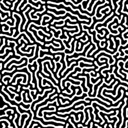In this article I will talk about one unusual approach to the generation of labyrinths. It is based on the Amarí model of the neural activity of the cerebral cortex, which is a continuous analogue of neural networks. Under certain conditions, it allows you to create beautiful labyrinths of a very complex shape, similar to the one shown in the picture.

You will find a lot of analysis and some private derivatives. The code is attached.
I ask under the cat!

Introduction

Many of the readers have already encountered the task of generating the maze in one form or another and know that to solve it, they often use the Prima and Kruskal algorithms for finding the minimum spanning tree in a graph whose vertices are cells of the maze and the edges represent the passages between neighboring cells. We will take a bold step away from graph theory in the direction of ... computational neuroscience.
')
During the 20th century, scientists built mathematical models of single neurons (cells of the nervous system) and their interaction with each other. In 1975, S. Amari presented his continuous model of the cerebral cortex to light. In it, the nervous system was considered as a continuous medium, at each point of which there is a “neuron” characterized by the value of the potential of its membrane, which changes its potential, exchanging charges with neighboring neurons and external stimuli. The Amari model is famous for explaining many of the phenomena of human vision and, in particular, visual hallucinations caused by psychoactive substances.

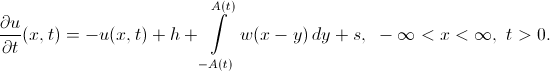
The Amari model, in its simplest form, is a Cauchy problem for a single integro-differential equation:

We can not do without explanations:

• - the real value of the membrane potential of the neuron at the point at the moment of time .
• - rest potential (some real constant).
• - Heviside step function:

  

• - weight function.
• - external irritant.
• - distribution of potential at the initial moment of time.
• - arbitrary point of the area on which potential is defined. Since we plan to generate a two-dimensional image of the maze, as We will consider the whole real plane.
• Partial derivative time in the left part indicates instantaneous change in potential . The right side sets the rule for this change.
• The first two components of the right-hand side mean that in the absence of stimuli, the value of the potential tends to the value of the rest potential.
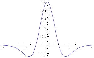
• The following term takes into account the effects of neighboring neurons. The Heviside function plays the role of the neuron's activation function: the neuron begins to influence its neighbors only if its potential is greater than zero. We will further call such neurons active, and the set of points with a positive potential - the area of ​​activity. It is clear that resting neurons should not be active, that is, the resting potential should not be positive. Active neighbors can be divided into two groups: stimulating and inhibiting. Excitating neurons increase the potential of neighbors, while inhibitory ones decrease it. At the same time, the exciters create a powerful surge of activity in a small neighborhood, and those who slow down are gradually quenching the activity in a neighborhood of a large radius. This fact is reflected in the choice of the weight function. in the form of "Mexican hat":

  
  

• The last term of the right side of the equation takes into account the action of an external stimulus. For example, for the visual cortex, a natural stimulus is a signal received from the retina. We assume that the stimulus is given by a nonnegative stationary (independent of time) function.

Let us ask ourselves: is it possible to choose the parameters of the model? so that its stationary solution (with ) was the image of some maze?

Properties of solutions of the Amari model

To analyze the solutions of the Amari model, it will be sufficient for us to restrict ourselves to the consideration of the one-dimensional case. For simplicity, we will assume that constant on the whole line.
First of all, we are interested in so-called bump solutions. They are remarkable in that they are positive only on a certain finite interval. with moving borders. The Amari equation for them is written as follows:

To understand how his decision behaves, we introduce the function

Now the same equation can be rewritten as:

We know that the bump solution vanishes at the boundaries of the interval of activity (because they are called boundaries). We write this condition on the right border:

And now we differentiate the last identity by variable :

From here:

Substituting the last expression into the equation for the bump solution when , we get:

Now we note that the partial derivative with respect to the left side is always negative, since the solution to the left of the right border is greater than zero, and to the right of it is smaller. therefore

Thus, the direction of the boundary shift depends only on the value of the expression on the right-hand side. If it is greater than zero, then the area of ​​activity expands; if it is less, it narrows. With zero equilibrium is achieved.
Take a look at the possible graphs of the function. .

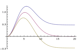
Obviously, two cases are possible:

1. Limit value non-negative. Then the area of ​​activity of the bump solution will expand indefinitely.
2. Limit value negatively. Then the area of ​​activity will be limited. Moreover, in this case, it can be shown that the connected components of the activity region of the solution of the Amari equation never merge .

Unfortunately, in the two-dimensional case, to obtain an explicit expression for the function difficult, so we just appreciate it:

From here:

Maze Generation

Having collected the necessary knowledge, we can proceed to the algorithm for generating a maze.
First of all, we will define the very concept of "labyrinth". By maze we mean binary function. such that area connected. A value of 0 corresponds to a free cell, and a value of 1 corresponds to an impassable wall. The condition of connectivity suggests that from any free cell one can get to any other without destroying the wall. Function we will look in the form:

Where - solution model Amari. It remains only to determine the parameters of the model.
Let's start with fixing an arbitrary negative value. . Naturally put . Now let's set the function . Let its value at each point is determined by a random variable uniformly distributed on the segment . In this case, the stimulus will not create activity. Fix an arbitrary positive . This parameter affects only the absolute value of the potential, therefore it is of no interest. We fix arbitrary positive ones. . They determine the characteristic thickness of the walls of the maze. Parameter We will try to determine experimentally, and then compare with the theoretical estimate obtained in the previous section.
The stationary solution will be sought by the method of successive approximations:

And here is the long-awaited interactive demonstration in Python:

import math import numpy import pygame from scipy.misc import imsave from scipy.ndimage.filters import gaussian_filter class AmariModel(object): def __init__(self, size): self.h = -0.1 self.k = 0.05 self.K = 0.125 self.m = 0.025 self.M = 0.065 self.stimulus = -self.h * numpy.random.random(size) self.activity = numpy.zeros(size) + self.h self.excitement = numpy.zeros(size) self.inhibition = numpy.zeros(size) def stimulate(self): self.activity[:, :] = self.activity > 0 sigma = 1 / math.sqrt(2 * self.k) gaussian_filter(self.activity, sigma, 0, self.excitement, "wrap") self.excitement *= self.K * math.pi / self.k sigma = 1 / math.sqrt(2 * self.m) gaussian_filter(self.activity, sigma, 0, self.inhibition, "wrap") self.inhibition *= self.M * math.pi / self.m self.activity[:, :] = self.h self.activity[:, :] += self.excitement self.activity[:, :] -= self.inhibition self.activity[:, :] += self.stimulus class AmariMazeGenerator(object): def __init__(self, size): self.model = AmariModel(size) pygame.init() self.display = pygame.display.set_mode(size, 0) pygame.display.set_caption("Amari Maze Generator") def run(self): pixels = pygame.surfarray.pixels3d(self.display) index = 0 running = True while running: self.model.stimulate() pixels[:, :, :] = (255 * (self.model.activity > 0))[:, :, None] pygame.display.flip() for event in pygame.event.get(): if event.type == pygame.QUIT: running = False elif event.type == pygame.KEYDOWN: if event.key == pygame.K_ESCAPE: running = False elif event.key == pygame.K_s: imsave("{0:04d}.png".format(index), pixels[:, :, 0]) index = index + 1 elif event.type == pygame.MOUSEBUTTONDOWN: position = pygame.mouse.get_pos() self.model.activity[position] = 1 pygame.quit() def main(): generator = AmariMazeGenerator((512, 512)) generator.run() if __name__ == "__main__": main() 

I suppose that comments are superfluous. I would like to note only that the convolution with the weight function is calculated through a Gaussian filter, and the images continue periodically to the whole plane (the “wrap” parameter). The demonstration is interactive in the sense that it allows you to forcibly establish a positive potential at any point on click.
The behavior of the solution, as expected, depends on the choice of the parameter. :

Now we get a theoretical estimate of the optimal value of the parameter . It satisfies the condition:

Therefore, it can be estimated as follows:

Not bad, but real value just above the theoretical estimate. This is easily seen by putting .

Finally, you can change the degree of "sparseness" of the maze by changing the value of the parameter :

Conclusion

So we have finished considering, perhaps, the most unusual way of generating labyrinths. I hope that the article seemed interesting to you. In conclusion, I will provide a list of references for those who want to expand their horizons:

[1] Konstantin Doubrovinski, Dynamics, Stability and Bifurcation Phenomena in the Nonlocal Model of Cortical Activity , 2005.
[2] Dequan Jin, Dong Liang, Jigen Peng, 2011.
[3] Stephen Coombes, Helmut Schmidt, Ingo Bojak, Interface Dynamics in Planar Neural Field Models , 2012.