Choosing a tool for floating-point calculations - practical tips
A modern programmer, mathematics or analytics often has to design, or even create software and hardware complexes for working with large arrays of numerical data. Building simulation models, forecasting, calculating statistics, managing operational processes, financial analysis, processing experimental data - everywhere you want to get the maximum calculation speed per unit of costs.
At the same time, most well, at least minimally complex and functional systems (in any case, of those that I personally met during 8 years of work in the banking sector) are usually heterogeneous — they consist of many functional blocks, like a motley sewn patchwork quilt, where Each shred is performed by a different application, often even on different hardware platforms. Why? Yes, it's just rational and convenient. Each product is good in its field. For example, economists like to use Ms Excel to analyze and visualize data. But few people would think of using this program to train serious artificial neural networks or solve real-time differential equations - for this, powerful universal packages offering flexible API are often purchased (or already acquired by the company), or individual modules are written to order. So it turns out that the result is considered more profitable in the same Matlab, stored in Oracle DBMS tables (running on a Linux cluster), and the report is shown to users in Excel, running as an OLE server on Windows. Moreover, all these components are connected by one of the universal programming languages.
How to choose the optimal implementation environment for a specific task? You encounter a compromise: some tools or libraries are more familiar to you, others have more functionality (say, support OOP), others have an advantage in execution speed (for example, use SSE-vectorization, like C ++), fourth provide high speed of development (for example, Visual Basic). The market today offers an impressive amount of both software tools - compilers, computer math systems, office suites, and hardware technologies (x86-x64, Cell, GPGPU) and tools for organizing their collaboration (networks, clusters, cloud computing).
')
Add to this trends in the use of computing resources (mass transition to parallel computing, application and server virtualization), new models of providing computing power (such as Amazon EC2), new methods for ensuring fault tolerance, licensing nuances - and you will get a huge number of combinations. How to choose the best?
The main recommendation is to first make a prototype in an environment with the fastest development speed, then move to a more time consuming option, trying to improve performance metrics (for example, reduce execution time) until you have exhausted the time limit for solving this subtask. At the same time, it is not worth spending energy on a deliberately unscaled solution. Do not be lazy, be sure to write the code and test it "live" by checking your guesses. Theoretical knowledge and sensitive intuition is fine, but very often the reality is different from our models and ideas, as you will see in my experience of solving a small production problem.
The other day I needed to optimize the implementation of a simple algorithm: calculating the sum of the sines of all the integers from 1 to two hundred million. Actually, of course, the real algorithm was somewhat different, but I was looking for the optimal tool for solving a similar class of problems; to build a complete infrastructure in each prototype at the initial stage did not make sense, so I simplified the algorithm to the limit. If you are wondering why such algorithms may be needed, let me remind you that trigonometric functions can be used, for example, as threshold activation functions for artificial neural networks. Spoiler: the results of the study were for me a complete surprise!
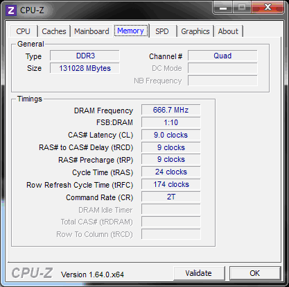
Workbench: Dual Xeon E5 2670 @ 2.6 Ghz with power-saving technology turned on, reducing the frequency of the CPU during idle time, 2x8 physical cores with hypertreading, 128 Gb DDR3-1600 memory on the Windows Server 2008R2 platform.

Double precision (double, i.e., one of the standard x86 coprocessor formats) to begin with will completely satisfy us. Let's see how different compilers, and then different computational architectures, will cope with the task of calculating the amount of sines. The race includes: Maple 12, Maple 17, MatLab R2013a, Visual Basic 6.0, Visual Basic .NET and Visual C ++ 2012 (in general, those who are at hand). All time measurements are made after the restart, and correspond to the average elapsed time.
I know, the testing technique is not the most stringent - just one type of processor, one OS, a simplified method of measuring performance. However, we do not have a scientific article, so we confine ourselves to the most interesting facts. I will not go into the details of the organization of intercomponent communications (as a rule, for Win there are enough components of COM and ordinary dll, well, and shared access to memory), just see what combination allows you to quickly calculate the desired result. First, let's find out which tool will generate the fastest single-threaded version, and then parallelize it, okay?
Maple 12 result:
1.25023042417602160 in 54.304 seconds
Maple 17 result:
1.25023042417610020 in 19.656 seconds
At first glance, the excellent work of MapleSoft engineers. 75% improved lead time from version to version of the product. Let's see if the 17th version can also compile this procedure. Naively calling
we get a procedure that for some reason gives zero in any case. We try alternative - an explicit cycle.
If you run p2 without compilation, the result can not wait! At least I waited 10 minutes and gave up. Apparently, for the Maple runtime, the sum function is significantly optimized compared to the loop. though
in Maple 17 gives excellent results:
1.25023042417610020 in 9.360 seconds!
Despite the "quirks" of the system, showing persistence and ingenuity, we were able to get an excellent performance boost :-)
I remember well how at one time I was deeply disappointed by the Net platform with the awful slowness of my compiled code. My test case (compiled!) In VB.Net 2003 ran 8 times slower than the code on VB6, so I didn’t have any special illusions collecting the project under VB.Net 2012.
As it turned out, nothing!
VB.Net 2012 result:
1.25023042417527 in 11.980 seconds, not bad!
The main hope I, of course, laid on the optimizing compiler Visual C ++, going to compile into native executable code, without any Net-ovsky slag, the following procedure:
Keys used / O2 and / Ot:

Result of VC ++. Net 2012:
not at all impressed: 1.2502304241761002 in 11.404 seconds.
The code looks very simple:
Compile with maximum optimization:

And we get the champion in the face of VB6:
Result: 1.25023042417543, Time spent: 0:00:09 (9.092153)
Now explain to me how the 12-year-old product makes new compilers in all respects ?! It seems that MS is degrading, but this is a topic for another conversation. If you look at the disassembler listing, you can see that the VC ++ compiler honestly vectorized the code:

True, I do not know the details of this implementation of sines on SSE2, but what is the use of it if it loses to the stack-based single-operand FPU commands that Visual Basic 6 used? I will tell you a secret, after such an unpleasant discovery, I downloaded a trial version of Intel Parallel Studio XE 2013 and rebuilt the project in the Intel C ++ 13 compiler with QxSSE4.2 keys, and then QxAVX - the results became even worse, in the region of 13-15 seconds. After such results a wild thought arose - or maybe not everything is in order with the processors of my server? I started comparing VB6 and VC ++ 2012 on another machine, an old Core Duo 6600 with two cores. The lag of the SSE version is even greater. The only logical explanation is that since the Core architecture, Intel engineers have significantly improved the performance of FPU operations compared to SSE, and the developers of the Microsoft and Intel compilers have lost sight of this fact.
In the picture above, by the way, you could observe that the Vtune Amplifier profiler in the Hot Spots mode did not cope with the timing calculation for SSE instructions. If you believe him, then the most time consuming operation in my code is an increase in the loop counter! Out of academic interest, since the Intel package was installed, I drove the module through Advisor XE 2013, a product designed to show places in the code that can be parallelized. In a short cycle without data dependencies, without shared resources, IDEALLY suitable for parallel execution, this product could not find such places. Well, how to trust this program in more difficult cases? Increasingly, there is a feeling that Intel programmers are releasing products, although they are well-advertised, but of little use for practice (and not only programmers, if we recall the corn announcements and re-announcements of Larrabee and Knights Corner). Well, we still have Matlab.
Typing
almost immediately see the result:
1.250230424175050, Elapsed time is 3.621641 seconds.
Well well! It turned out that smart Matlab immediately parallelized this expression by the number of physical cores on my local machine, ensuring their full load. Nice, isn't it? After all, I paid for powerful hardware and I would like the software (by the way, also not cheap) to use it 100%. Respect to MathWorks engineers!
Let's try to compile? To do this, transfer the expression to the m-file. And here we are waiting for another surprise. Uncompiled tic; FastSum (200000000); toc; gives Elapsed time already 5.607512 seconds. Who has already encountered this, what is the matter? It's a mystery for me. We use the help of the deploytool command, wait a certain number of minutes, and Matlab creates for us a hefty executable in half a megabyte. Yeah, the compiler development team has more work to do - for comparison, the size of VC ++ is 46Kb, VB.Net is 30Kb, Vb6 is 36Kb. But what will the compiled Matlab executable give us?
1.2502, Elapsed time is 10.716620 seconds.
In the compiled version, as you can see, the automatic cycle parallelization for some reason disappears. My heart tells me that the company wants extra money for Parallel Computing Toolbox :-)
In any case, the leader is VB6, so I wrote a simple Active Exe server in this environment that allows us to parallelize our calculations for a given number of threads:

Let's see how well our solution scales with an increase in the number of workflows from 1 to 32. To be honest, I was sure that productivity would increase until it reaches the ceiling as the number of physical cores of processors, for whence the HT virtual cores take resources for does floating point work if the FPU pipeline is already fully occupied?

However, by additionally using 14 logical cores, we managed to reduce the execution time by 20%: from t (16) = 0.803 sec. to t (30) = 0.645. Perhaps the result would have been more impressive if the processors were not originally in the power saving mode, because in 0.6 seconds, it seems, they simply do not have time to increase the clock frequency to the maximum.
Well, we found the optimal solution for the mainstream configuration in our particular case. But let's not forget about GPGPU (graphics cards with the possibility of universal computing), which more and more servers are being equipped with today, and almost all home computers and new laptops are almost certainly equipped. My poster server was no exception - ex-flagship Nvidia, a dual-chip GTX 590 graphics card with Fermi architecture, supporting CUDA technology, was purchased specifically for multi-thread computing.
In general, I must say that I immensely respect Nvidia. First, for the fact that this is perhaps the only company that really promotes highly parallel computing to the masses (conferences, seminars, events, active development and improvement of software and architecture), and secondly, for the fact that it managed to organize sales of the specialized " iron "and take the lead in the new sector of high-performance computing. Yes, AMD (ATI) solutions are more powerful, AMD cards probably have more gigaflops, but you try to start development under FireStream - on the AMD website you will not find any sensible documentation or a clear description of the technology itself. It seems that AMD’s programmers / marketers / management simply buried the work of talented ATI engineers. So our choice is CUDA! By the way, if you have problems with the integration of CUDA 5 and Visual Studio 2012, you can use the recommendations of this article.
So, what resources does our miracle device have?

As you can see, theoretically, we can run calculations in 16 * 1536 * 2 = 49152 threads on two GPU devices. In fact, everything is not so rosy - the sines in Fermi are considered in Special Functions Units, of which 4 are per multiprocessor (SM). Total we can count at the same time no more than 16 * 4 * 2 = 128 values (again, theoretically).
I would not like to go straight into the details of the CUDA architecture, especially in the subtleties of optimization for CUDA - this is both science and art in themselves. Therefore, let's start with a fast prototype in the Thrust library, designed to increase the productivity of programmers through the high level of abstraction of the CUDA model, in peak with the lower-level CUDA C.
The beauty of Thrust is that, according to the creators' assurances, developers no longer need to spend time on self-realization of such primitives as arithmetic operations, sorting, various reductions (a term that probably firmly entered the vocabulary of most programmers precisely after familiarizing themselves with the CUDA manuals) , search, reorganization of arrays and other types of operations. In addition, this library independently determines the optimal launch configuration, and you do not need to focus on determining the optimal ratio of the number of blocks and GPU threads, as before ...
Although Thrust does not automatically use all CUDA-compatible devices, it chooses the fastest one, in any case, I expected the unconditional victory of Nvidia number shredders, although I knew about the reduced performance in double-precision calculations. After all, one thing is to calculate two hundred million sines, you still need to effectively reduce the entire array to a single total value, with which highly parallel algorithms usually cope very well.
We will use the powerful transform_reduce function that allows you to transform and summarize the elements of an array in one logical step. We create for it a special functor sin_op. The code is quite simple:
I use an external loop to ensure that I get the right amount of memory on the device - sadly, Thrust does not always cope with this on its own. Logically, a thread should calculate its integer index, apply a transforming functor to it, and store the result in a fast shared memory. So, compile, run:
1.2502304241755013 in 1.704 seconds
There is no limit to frustration. The result of kakbe hints that the library makes the accelerator do not exactly what we have drawn in our imagination. Indeed, if you look at the detailed timings, it turns out that the library is trying to start with placing a huge array of zeros in the relatively slow main memory of the device (which it spends 35% of the time), then overwrites these zeros with the natural number 1,2,3 ... (40% time), well, the remaining 25% of the time is occupied with the calculation of sines and directly by summation (reduction by the plus operator, and also in slow main memory).
Having grieved, we remember that in this library there are virtual iterators (fancy iterators). We look in the documentation - well, exactly
What is the lead time? Reduced by almost half, getting rid of inefficient operations with the main memory:
1.2502304241761253 in 0.780 sec.
Here it should be taken into account that even an empty call of the device context with waiting takes some time, at least this time averaged 0.26 seconds from me. Be that as it may, even 0.52 seconds is not the result that you expect from a device of a massively parallel architecture with peak performance of several teraflops. Let's try to write a core on CUDA C, which will perform a preliminary summation. This is not so difficult ... Let us divide for this our calculations into blocks of equal length. Each block will carry out a parallel reduction of its elements in fast shared memory, and save the result to the accelerator's global memory, at an offset equal to the block index:
Theoretically, one block can sum up to 1024 items on our device. After the first call of the SumOfSinuses kernel, we will have about 200 thousand intermediate terms in the memory of the device, which can be easily folded with one call to thrust :: reduce:
1.2502304241758133 in 0.749 seconds
I have to use the Do cycle for the reason that the grid size of CUDA blocks is limited. Therefore, in our case, the kernel is called three times from the loop, each time processing approximately 70 million terms. It turns out that, after all, performance rests on calculating transcendental functions with double precision, so Thrust is not to blame for relatively poor performance, and I would advise using the first option, with a more understandable and elegant code. By the way, our approach is not yet scaled by the number of CUDA-compatible devices (of which a local cluster may well be organized). Can this be fixed? It turns out that a simple context switch between two devices and the entire auxiliary binding (call cudaSetDevice, cudaStreamCreate / cudaStreamDestroy) for some reason takes about 0.5 seconds. That is, it turns out that scaling across multiple CUDA devices is beneficial if the cores are running long enough so that the overhead of context switching is invisible. In our case, this is not the case, so we leave scaling on several devices beyond the scope of the article (perhaps I should have used several threads and on the host side, I'm not sure).
I almost forgot - after all, Matlab has been supporting the code execution on CUDA devices for three years already (of course, with some restrictions). Those interested can watch the English-language webinar (registration required). For the sake of objectivity, it should be noted that CUDA support is rudimentary in Maple, at the level of several procedures of a linear algebra package. MatLab in this regard is much more advanced. I do not know whether in the current version it is possible to fill arrays with sequences directly on the device, without copying arrays from the host (judging by the documentation, it is impossible). So let's apply a frontal approach:
1.250230424175708, Elapsed time is 2.872859 seconds.
Making the code work on both processors of my dual-chip accelerator did not work right away, in the manuals this topic is not fully disclosed. Spmd works, a composite array, divided into 2 parts, is created. However, at some point the program goes to error, reporting that the data is no longer available. Who has already worked with several GPUs in the hardware, respond ;-) In any case, the Matlab version will not be faster than our implementation in Thrust.
Well, I would like to take fasm and add another purely assembler version, optimized using Vtune event-based profiling for cache misses and other subtleties, but no longer strong :-) If there are volunteers, please send your results, I will gladly add an article. It would also be interesting to see the launch results under Knights Corner, but unfortunately there is no suitable hardware.
At the same time, most well, at least minimally complex and functional systems (in any case, of those that I personally met during 8 years of work in the banking sector) are usually heterogeneous — they consist of many functional blocks, like a motley sewn patchwork quilt, where Each shred is performed by a different application, often even on different hardware platforms. Why? Yes, it's just rational and convenient. Each product is good in its field. For example, economists like to use Ms Excel to analyze and visualize data. But few people would think of using this program to train serious artificial neural networks or solve real-time differential equations - for this, powerful universal packages offering flexible API are often purchased (or already acquired by the company), or individual modules are written to order. So it turns out that the result is considered more profitable in the same Matlab, stored in Oracle DBMS tables (running on a Linux cluster), and the report is shown to users in Excel, running as an OLE server on Windows. Moreover, all these components are connected by one of the universal programming languages.
How to choose the optimal implementation environment for a specific task? You encounter a compromise: some tools or libraries are more familiar to you, others have more functionality (say, support OOP), others have an advantage in execution speed (for example, use SSE-vectorization, like C ++), fourth provide high speed of development (for example, Visual Basic). The market today offers an impressive amount of both software tools - compilers, computer math systems, office suites, and hardware technologies (x86-x64, Cell, GPGPU) and tools for organizing their collaboration (networks, clusters, cloud computing).
')
Add to this trends in the use of computing resources (mass transition to parallel computing, application and server virtualization), new models of providing computing power (such as Amazon EC2), new methods for ensuring fault tolerance, licensing nuances - and you will get a huge number of combinations. How to choose the best?
The main recommendation is to first make a prototype in an environment with the fastest development speed, then move to a more time consuming option, trying to improve performance metrics (for example, reduce execution time) until you have exhausted the time limit for solving this subtask. At the same time, it is not worth spending energy on a deliberately unscaled solution. Do not be lazy, be sure to write the code and test it "live" by checking your guesses. Theoretical knowledge and sensitive intuition is fine, but very often the reality is different from our models and ideas, as you will see in my experience of solving a small production problem.
The other day I needed to optimize the implementation of a simple algorithm: calculating the sum of the sines of all the integers from 1 to two hundred million. Actually, of course, the real algorithm was somewhat different, but I was looking for the optimal tool for solving a similar class of problems; to build a complete infrastructure in each prototype at the initial stage did not make sense, so I simplified the algorithm to the limit. If you are wondering why such algorithms may be needed, let me remind you that trigonometric functions can be used, for example, as threshold activation functions for artificial neural networks. Spoiler: the results of the study were for me a complete surprise!
Formulation of the problem:
Workbench: Dual Xeon E5 2670 @ 2.6 Ghz with power-saving technology turned on, reducing the frequency of the CPU during idle time, 2x8 physical cores with hypertreading, 128 Gb DDR3-1600 memory on the Windows Server 2008R2 platform.
Double precision (double, i.e., one of the standard x86 coprocessor formats) to begin with will completely satisfy us. Let's see how different compilers, and then different computational architectures, will cope with the task of calculating the amount of sines. The race includes: Maple 12, Maple 17, MatLab R2013a, Visual Basic 6.0, Visual Basic .NET and Visual C ++ 2012 (in general, those who are at hand). All time measurements are made after the restart, and correspond to the average elapsed time.
I know, the testing technique is not the most stringent - just one type of processor, one OS, a simplified method of measuring performance. However, we do not have a scientific article, so we confine ourselves to the most interesting facts. I will not go into the details of the organization of intercomponent communications (as a rule, for Win there are enough components of COM and ordinary dll, well, and shared access to memory), just see what combination allows you to quickly calculate the desired result. First, let's find out which tool will generate the fastest single-threaded version, and then parallelize it, okay?
Let's start with Maple:
st := time():evalhf(sum(sin(i),i=1..200000000));time() - st; Maple 12 result:
1.25023042417602160 in 54.304 seconds
Maple 17 result:
1.25023042417610020 in 19.656 seconds
At first glance, the excellent work of MapleSoft engineers. 75% improved lead time from version to version of the product. Let's see if the 17th version can also compile this procedure. Naively calling
cp:=Compiler:-Compile(proc(j::integer)::float;local i::integer: evalhf(sum(sin(i),i=1..j)) end proc:): we get a procedure that for some reason gives zero in any case. We try alternative - an explicit cycle.
p2 := proc(j::integer)::float;local i::integer,res::float;res:=0; for i from 1 to j do: res:=res+evalhf(sin(i)):end do; res end proc: If you run p2 without compilation, the result can not wait! At least I waited 10 minutes and gave up. Apparently, for the Maple runtime, the sum function is significantly optimized compared to the loop. though
cp2:=Compiler:-Compile(p2): st := time():cp2(200000000);time() - st; in Maple 17 gives excellent results:
1.25023042417610020 in 9.360 seconds!
Despite the "quirks" of the system, showing persistence and ingenuity, we were able to get an excellent performance boost :-)
Moving on to Microsoft Visual Studio 2012
I remember well how at one time I was deeply disappointed by the Net platform with the awful slowness of my compiled code. My test case (compiled!) In VB.Net 2003 ran 8 times slower than the code on VB6, so I didn’t have any special illusions collecting the project under VB.Net 2012.
Public Class Form1 Private Sub Form1_Load(sender As Object, e As EventArgs) Handles MyBase.Load Dim i As Long, res As Double, tm As DateTime tm = Now For i = 1 To 200000000 res = res + Math.Sin(i) Next TextBox1.Text = res & vbNewLine & Now.Subtract(tm).TotalSeconds.ToString("0.000") End Sub End Class As it turned out, nothing!
VB.Net 2012 result:
1.25023042417527 in 11.980 seconds, not bad!
The main hope I, of course, laid on the optimizing compiler Visual C ++, going to compile into native executable code, without any Net-ovsky slag, the following procedure:
#include <iostream> #include <windows.h> using namespace std; int main() { double res=0.0; int dw = GetTickCount(); for (int i = 1; i <= 200000000; i++) res+=sin(i); cout.precision(20); cout << "Result: " << res << " after " << (GetTickCount()-dw); } Keys used / O2 and / Ot:
Result of VC ++. Net 2012:
not at all impressed: 1.2502304241761002 in 11.404 seconds.
It's the turn of the old school VB6
The code looks very simple:
res = 0: for i = 1 To 200000000: res = res + Sin(i) : Next i Compile with maximum optimization:
And we get the champion in the face of VB6:
Result: 1.25023042417543, Time spent: 0:00:09 (9.092153)
Now explain to me how the 12-year-old product makes new compilers in all respects ?! It seems that MS is degrading, but this is a topic for another conversation. If you look at the disassembler listing, you can see that the VC ++ compiler honestly vectorized the code:
True, I do not know the details of this implementation of sines on SSE2, but what is the use of it if it loses to the stack-based single-operand FPU commands that Visual Basic 6 used? I will tell you a secret, after such an unpleasant discovery, I downloaded a trial version of Intel Parallel Studio XE 2013 and rebuilt the project in the Intel C ++ 13 compiler with QxSSE4.2 keys, and then QxAVX - the results became even worse, in the region of 13-15 seconds. After such results a wild thought arose - or maybe not everything is in order with the processors of my server? I started comparing VB6 and VC ++ 2012 on another machine, an old Core Duo 6600 with two cores. The lag of the SSE version is even greater. The only logical explanation is that since the Core architecture, Intel engineers have significantly improved the performance of FPU operations compared to SSE, and the developers of the Microsoft and Intel compilers have lost sight of this fact.
In the picture above, by the way, you could observe that the Vtune Amplifier profiler in the Hot Spots mode did not cope with the timing calculation for SSE instructions. If you believe him, then the most time consuming operation in my code is an increase in the loop counter! Out of academic interest, since the Intel package was installed, I drove the module through Advisor XE 2013, a product designed to show places in the code that can be parallelized. In a short cycle without data dependencies, without shared resources, IDEALLY suitable for parallel execution, this product could not find such places. Well, how to trust this program in more difficult cases? Increasingly, there is a feeling that Intel programmers are releasing products, although they are well-advertised, but of little use for practice (and not only programmers, if we recall the corn announcements and re-announcements of Larrabee and Knights Corner). Well, we still have Matlab.
The experiment with Matlab pleasantly surprised
Typing
tic;sum(sin(1:200000000));toc; almost immediately see the result:
1.250230424175050, Elapsed time is 3.621641 seconds.
Well well! It turned out that smart Matlab immediately parallelized this expression by the number of physical cores on my local machine, ensuring their full load. Nice, isn't it? After all, I paid for powerful hardware and I would like the software (by the way, also not cheap) to use it 100%. Respect to MathWorks engineers!
Let's try to compile? To do this, transfer the expression to the m-file. And here we are waiting for another surprise. Uncompiled tic; FastSum (200000000); toc; gives Elapsed time already 5.607512 seconds. Who has already encountered this, what is the matter? It's a mystery for me. We use the help of the deploytool command, wait a certain number of minutes, and Matlab creates for us a hefty executable in half a megabyte. Yeah, the compiler development team has more work to do - for comparison, the size of VC ++ is 46Kb, VB.Net is 30Kb, Vb6 is 36Kb. But what will the compiled Matlab executable give us?
1.2502, Elapsed time is 10.716620 seconds.
In the compiled version, as you can see, the automatic cycle parallelization for some reason disappears. My heart tells me that the company wants extra money for Parallel Computing Toolbox :-)
In any case, the leader is VB6, so I wrote a simple Active Exe server in this environment that allows us to parallelize our calculations for a given number of threads:
Let's see how well our solution scales with an increase in the number of workflows from 1 to 32. To be honest, I was sure that productivity would increase until it reaches the ceiling as the number of physical cores of processors, for whence the HT virtual cores take resources for does floating point work if the FPU pipeline is already fully occupied?
However, by additionally using 14 logical cores, we managed to reduce the execution time by 20%: from t (16) = 0.803 sec. to t (30) = 0.645. Perhaps the result would have been more impressive if the processors were not originally in the power saving mode, because in 0.6 seconds, it seems, they simply do not have time to increase the clock frequency to the maximum.
GPGPU
Well, we found the optimal solution for the mainstream configuration in our particular case. But let's not forget about GPGPU (graphics cards with the possibility of universal computing), which more and more servers are being equipped with today, and almost all home computers and new laptops are almost certainly equipped. My poster server was no exception - ex-flagship Nvidia, a dual-chip GTX 590 graphics card with Fermi architecture, supporting CUDA technology, was purchased specifically for multi-thread computing.
In general, I must say that I immensely respect Nvidia. First, for the fact that this is perhaps the only company that really promotes highly parallel computing to the masses (conferences, seminars, events, active development and improvement of software and architecture), and secondly, for the fact that it managed to organize sales of the specialized " iron "and take the lead in the new sector of high-performance computing. Yes, AMD (ATI) solutions are more powerful, AMD cards probably have more gigaflops, but you try to start development under FireStream - on the AMD website you will not find any sensible documentation or a clear description of the technology itself. It seems that AMD’s programmers / marketers / management simply buried the work of talented ATI engineers. So our choice is CUDA! By the way, if you have problems with the integration of CUDA 5 and Visual Studio 2012, you can use the recommendations of this article.
So, what resources does our miracle device have?
As you can see, theoretically, we can run calculations in 16 * 1536 * 2 = 49152 threads on two GPU devices. In fact, everything is not so rosy - the sines in Fermi are considered in Special Functions Units, of which 4 are per multiprocessor (SM). Total we can count at the same time no more than 16 * 4 * 2 = 128 values (again, theoretically).
I would not like to go straight into the details of the CUDA architecture, especially in the subtleties of optimization for CUDA - this is both science and art in themselves. Therefore, let's start with a fast prototype in the Thrust library, designed to increase the productivity of programmers through the high level of abstraction of the CUDA model, in peak with the lower-level CUDA C.
The beauty of Thrust is that, according to the creators' assurances, developers no longer need to spend time on self-realization of such primitives as arithmetic operations, sorting, various reductions (a term that probably firmly entered the vocabulary of most programmers precisely after familiarizing themselves with the CUDA manuals) , search, reorganization of arrays and other types of operations. In addition, this library independently determines the optimal launch configuration, and you do not need to focus on determining the optimal ratio of the number of blocks and GPU threads, as before ...
Although Thrust does not automatically use all CUDA-compatible devices, it chooses the fastest one, in any case, I expected the unconditional victory of Nvidia number shredders, although I knew about the reduced performance in double-precision calculations. After all, one thing is to calculate two hundred million sines, you still need to effectively reduce the entire array to a single total value, with which highly parallel algorithms usually cope very well.
We will use the powerful transform_reduce function that allows you to transform and summarize the elements of an array in one logical step. We create for it a special functor sin_op. The code is quite simple:
#include <thrust/transform_reduce.h> #include <thrust/device_vector.h> #include <thrust/host_vector.h> #include <thrust/functional.h> #include <thrust/sequence.h> #include <windows.h> using namespace std; template <typename T> struct sin_op { __host__ __device__ T operator()(const T& x) const { return sin(x); } }; int main(void) { int dw = GetTickCount(); int n=10; double res=0.0; sin_op<double> tr_op; thrust::plus<double> red_op; thrust::device_vector<int> i(200000000/n); for (int j=1;j<=n;j++) { thrust::sequence(i.begin(), i.end(),200000000/n*(j-1)+1); res = thrust::transform_reduce(i.begin(), i.end(), tr_op, res, red_op); } cout.precision(20); cout << res << endl<< "Total Time: " << (GetTickCount()-dw) << endl; } I use an external loop to ensure that I get the right amount of memory on the device - sadly, Thrust does not always cope with this on its own. Logically, a thread should calculate its integer index, apply a transforming functor to it, and store the result in a fast shared memory. So, compile, run:
1.2502304241755013 in 1.704 seconds
There is no limit to frustration. The result of kakbe hints that the library makes the accelerator do not exactly what we have drawn in our imagination. Indeed, if you look at the detailed timings, it turns out that the library is trying to start with placing a huge array of zeros in the relatively slow main memory of the device (which it spends 35% of the time), then overwrites these zeros with the natural number 1,2,3 ... (40% time), well, the remaining 25% of the time is occupied with the calculation of sines and directly by summation (reduction by the plus operator, and also in slow main memory).
Having grieved, we remember that in this library there are virtual iterators (fancy iterators). We look in the documentation - well, exactly
While constant_iterator and counting_iterator act as arrays, they don’t really need any memory storage. Whenever we dereference one of these iterators.The counting iterator is what the doctor ordered:
#include <thrust/iterator/counting_iterator.h> #include <thrust/transform_reduce.h> #include <thrust/device_vector.h> #include <thrust/host_vector.h> #include <thrust/functional.h> #include <thrust/sequence.h> #include <windows.h> using namespace std; template <typename T> struct sin_op { __host__ __device__ T operator()(const T& x) const { return sin(x); } }; int main(void) { int dw = GetTickCount(); double res=0.0; sin_op<double> tr_op; thrust::plus<double> red_op; thrust::counting_iterator<int> first(1); thrust::counting_iterator<int> last = first + 200000000; res = thrust::transform_reduce(first, last, tr_op, res, red_op); cout.precision(20); cout << res << endl<< "Total Time: " << (GetTickCount()-dw)<< endl; } What is the lead time? Reduced by almost half, getting rid of inefficient operations with the main memory:
1.2502304241761253 in 0.780 sec.
Here it should be taken into account that even an empty call of the device context with waiting takes some time, at least this time averaged 0.26 seconds from me. Be that as it may, even 0.52 seconds is not the result that you expect from a device of a massively parallel architecture with peak performance of several teraflops. Let's try to write a core on CUDA C, which will perform a preliminary summation. This is not so difficult ... Let us divide for this our calculations into blocks of equal length. Each block will carry out a parallel reduction of its elements in fast shared memory, and save the result to the accelerator's global memory, at an offset equal to the block index:
__global__ void SumOfSinuses(double *partial_res, int n) { // extern- extern __shared__ double sdata[]; // int i =blockIdx.x*blockDim.x+threadIdx.x; sdata[threadIdx.x] = (i <= n) ? sin((double)i) : 0; __syncthreads(); // for (int s=blockDim.x/2; s>0; s>>=1) { if (threadIdx.x < s) { sdata[threadIdx.x] += sdata[threadIdx.x + s]; } __syncthreads(); } // , if (threadIdx.x == 0) partial_res[blockIdx.x] = sdata[0]; } Theoretically, one block can sum up to 1024 items on our device. After the first call of the SumOfSinuses kernel, we will have about 200 thousand intermediate terms in the memory of the device, which can be easily folded with one call to thrust :: reduce:
int main(void) { int dw = GetTickCount(); int N=200000000+1; cudaDeviceProp deviceProp; cudaGetDeviceProperties(&deviceProp, 0); double *partial_res; int rest=N;int i=0;double res=0; int threads_per_block=1024;//deviceProp.maxThreadsPerBlock; int max_ind=deviceProp.maxGridSize[0] * threads_per_block; checkCudaErrors(cudaMalloc(&partial_res, max_ind/threads_per_block*sizeof(double))); thrust::device_ptr<double> arr_ptr(partial_res); do { int num_blocks=min((min(rest,max_ind) % threads_per_block==0) ? min(rest,max_ind)/threads_per_block : min(rest,max_ind)/threads_per_block+1,deviceProp.maxGridSize[0]); SumOfSinuses<<<num_blocks,threads_per_block,threads_per_block*sizeof(double)>>>(partial_res,i*max_ind,N); checkCudaErrors(cudaDeviceSynchronize()); // thrust- , res = thrust::reduce(arr_ptr, arr_ptr+num_blocks,res); rest -=num_blocks*threads_per_block; i++; } while (rest>0); cudaFree(partial_res); cout.precision(20); cout << res << endl<< "Total Time: " << (GetTickCount()-dw)<< endl; } 1.2502304241758133 in 0.749 seconds
I have to use the Do cycle for the reason that the grid size of CUDA blocks is limited. Therefore, in our case, the kernel is called three times from the loop, each time processing approximately 70 million terms. It turns out that, after all, performance rests on calculating transcendental functions with double precision, so Thrust is not to blame for relatively poor performance, and I would advise using the first option, with a more understandable and elegant code. By the way, our approach is not yet scaled by the number of CUDA-compatible devices (of which a local cluster may well be organized). Can this be fixed? It turns out that a simple context switch between two devices and the entire auxiliary binding (call cudaSetDevice, cudaStreamCreate / cudaStreamDestroy) for some reason takes about 0.5 seconds. That is, it turns out that scaling across multiple CUDA devices is beneficial if the cores are running long enough so that the overhead of context switching is invisible. In our case, this is not the case, so we leave scaling on several devices beyond the scope of the article (perhaps I should have used several threads and on the host side, I'm not sure).
I almost forgot - after all, Matlab has been supporting the code execution on CUDA devices for three years already (of course, with some restrictions). Those interested can watch the English-language webinar (registration required). For the sake of objectivity, it should be noted that CUDA support is rudimentary in Maple, at the level of several procedures of a linear algebra package. MatLab in this regard is much more advanced. I do not know whether in the current version it is possible to fill arrays with sequences directly on the device, without copying arrays from the host (judging by the documentation, it is impossible). So let's apply a frontal approach:
tic; res=0.0;n=10;stride=200000000/n; for j=1:n X=stride*(j-1)+1:stride*j; A=gpuArray(X); res=res+sum(sin(A)); end toc; gather(res) 1.250230424175708, Elapsed time is 2.872859 seconds.
Making the code work on both processors of my dual-chip accelerator did not work right away, in the manuals this topic is not fully disclosed. Spmd works, a composite array, divided into 2 parts, is created. However, at some point the program goes to error, reporting that the data is no longer available. Who has already worked with several GPUs in the hardware, respond ;-) In any case, the Matlab version will not be faster than our implementation in Thrust.
Well, I would like to take fasm and add another purely assembler version, optimized using Vtune event-based profiling for cache misses and other subtleties, but no longer strong :-) If there are volunteers, please send your results, I will gladly add an article. It would also be interesting to see the launch results under Knights Corner, but unfortunately there is no suitable hardware.
And a bonus for those who read it to the very end.
Surely many have noticed that I cheated. A specific amount of sines can be obtained not only by summing 200 million numbers, but also by simple multiplication of several quantities, if we note that

Well, or not to notice, but to drive in a symbolic form the formula in Mathematica or Maple. The required number with 50 exact decimal places:
The most important and the first optimization is always at the algorithm level :-) However, the work done was not useless - after all, a more complex pattern would most likely not allow the use of an analytical formula, but we already figured out how to cope with numerical tasks. By the way, if the accuracy of summation is important, additional measures should be taken to avoid losing significant figures when adding small terms to a large total amount — for example, use the Kagan algorithm. I hope you were interested!
Respectfully,
Anatoly Alekseev
05.24.2013
Well, or not to notice, but to drive in a symbolic form the formula in Mathematica or Maple. The required number with 50 exact decimal places:
1.2502304241756868163500362795713040947699040278200 The most important and the first optimization is always at the algorithm level :-) However, the work done was not useless - after all, a more complex pattern would most likely not allow the use of an analytical formula, but we already figured out how to cope with numerical tasks. By the way, if the accuracy of summation is important, additional measures should be taken to avoid losing significant figures when adding small terms to a large total amount — for example, use the Kagan algorithm. I hope you were interested!
Respectfully,
Anatoly Alekseev
05.24.2013
Source: https://habr.com/ru/post/181051/
All Articles