Hidden Markov chains, Viterbi algorithm
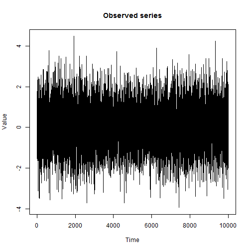
We need to implement a lie detector that, according to the shaking of a person’s hands, determines whether he is telling the truth or not. Suppose when a person lies, his hands are shaking a little more. The signal may be:
An interesting method is described in the article “A Tutorial on Hidden Markov Models and Selected Applications in Speech Recognition” by LR Rabiner, which introduces the Markov hidden circuit model and describes three valuable algorithms: The Forward-Backward Procedure , Viterbi Algorithm and Baum-Welch reestimation . Despite the fact that these algorithms are of interest only in the aggregate, for a better understanding, it is better to describe them separately.
')
The Markov hidden circuit method is widely used, for example, it is used to search for CG islands (DNA, high density cytosine and guanine RNA sections), while Lawrence Rabiner himself used it for speech recognition. The algorithms were useful to me in order to track the change of sleep / wake stages on the EEG and look for epileptic seizures.
In the model of hidden Markov chains, it is assumed that the system under consideration has the following properties:
The HMM model can be described as:
Time t is assumed to be discrete, given by non-negative integers, where 0 corresponds to the initial moment of time, and Tm is the highest value.
When we have 2 hidden states, and the observed values obey the normal distribution with different variances, as in the example with the lie detector, for each of the states, the system functioning algorithm can be depicted like this:

A simpler description was already mentioned in Probabilistic models: examples and pictures .
The choice of the vector of distributions of observable quantities often lies with the researcher. Ideally, the observed value is the hidden state, and the task of determining these states in this case becomes trivial. In reality, the classical model described by Rabiner, for example, is becoming more complex. - final discrete distribution. Something like what is on the chart below:
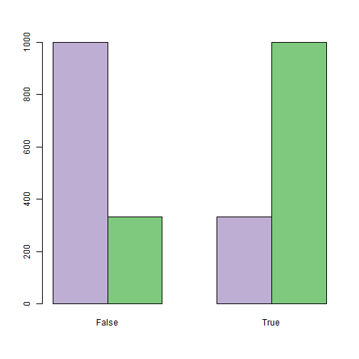
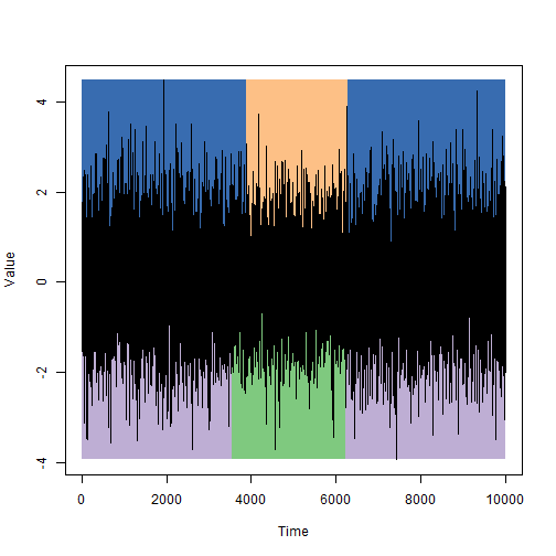
The researcher usually has the freedom to choose the distribution of the observed states. The stronger the observed values distinguish hidden states the better. From a programming point of view, going through the various observables means that you need to carefully encapsulate . The graph below shows an example of the source data for the lie detector problem, where the distribution of the observed characteristic (hand shake) is continuous, since it was modeled as normal with an average of 0 for both states, with a dispersion equal to 1, when a person tells the truth (purple columns) and 1.21 when lying (green columns):

In order not to touch on the issues of setting up the model, we consider a simplified problem.
Given:
two hidden states, where white noise with variance 1 corresponds to honest behavior, lies — white noise with dispersion 1.21;
sample of 10,000 consecutive observations o;
the change of state occurs on average once every 2,500 cycles.
It is required to determine the moments of change of states.
Decision:
Let's set the five parameters of the model:
Let us find the most plausible states for each moment of time using the Viterbi algorithm for the given model parameters.
The solution of the problem is reduced to specifying the model and running the Viterbi algorithm.
Using the model of hidden Markov chains and a sample of values of the observed characteristics, we find the sequence of states that best describes the sample in a given model. The concept can best be interpreted differently, but the well-established solution is the Viterbi algorithm, which finds such a sequence , what
  .
.
Search task is solved using dynamic programming, for this we consider the function:

Where - the highest probability of being able to s at the moment of time t. Recursively, this function can be defined as follows:

Simultaneously with the calculation for each moment of time we remember the most probable state from which we came, that is, 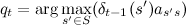 at which the maximum was reached. Wherein
  and that means you can recover
  , walking on them in reverse order. You may notice that
 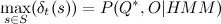 - the value of the desired probability. Required sequence found. An interesting feature of the algorithm is that the estimated function of the observed characteristics is included in in the form of a factor. If we assume that
  , then in the case of omissions in observations, it is still possible to estimate the most probable hidden states at these moments.
The “Pseudocode” for the Viterbi algorithm is sketched below. It should be noted that all operations with vectors and matrices are element-wise .
Someone could recognize the code in R in this “pseudocode”, but this is far from the best implementation.
Let us compare the periods of constancy of the states that were specified in the simulation (the upper part of the graph) and those that were found using the Viterbi algorithm (the lower part of the graph):
It is quite worthy in my opinion, but every time you should not hope for that.
The previously described Viterbi algorithm requires the definition of a hidden Markov chain model (Arguments of the viterbi function). To set them, a simple initialization is used, which implies that in addition to a sample of observable quantities O, a corresponding selection of hidden states Q, which we know from somewhere, is also given. In this case, the formulas for estimating the parameters will be as follows:
![S \ leftarrow \ left \ {s: q_t = s, t \ in [0, T_m] \ right \} \\ M \ leftarrow \ | S \ | \\ I \ leftarrow \ left (\ frac {\ sum_ {t \ in [0, T_m]} Id (q_t = s)} {T_m + 1}, s \ in S \ right) \\ T \ leftarrow \ left (\ frac {\ sum_ {t \ in [1, T_m]} Id (q_ {t-1} = s', q_t = s)} {\ sum_ {t \ in [0, T_m]} (\ sum_ { t \ in [1, T_m]} Id (q_ {t-1} = s ')}, s, s' \ in S \ right) \\ E \ leftarrow \ left (f_s (o_t) = \ frac {\ sum_ {t \ in [0, T_m]} Id (q_t = s, o_t = e)} {\ sum_ {t \ in [0, T_m]} Id (q_t = s)}, s \ in S \ right)](http://mathurl.com/ark5aup.png)
where Id (x) is an indicator function,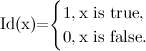
For the considered lie detector example, the algorithm incorrectly classified 413 out of 10,000 states (~ 4%), which is not bad at all. The Viterbi algorithm is able to accurately detect the moments of change of hidden states, but only if the distributions of the observed characteristics are accurately known. If only a parametric class of such distributions is known, then there is a way to select the most appropriate parameters, called the Baum-Welch algorithm.
If interested, ask to continue ...
An interesting method is described in the article “A Tutorial on Hidden Markov Models and Selected Applications in Speech Recognition” by LR Rabiner, which introduces the Markov hidden circuit model and describes three valuable algorithms: The Forward-Backward Procedure , Viterbi Algorithm and Baum-Welch reestimation . Despite the fact that these algorithms are of interest only in the aggregate, for a better understanding, it is better to describe them separately.
')
The Markov hidden circuit method is widely used, for example, it is used to search for CG islands (DNA, high density cytosine and guanine RNA sections), while Lawrence Rabiner himself used it for speech recognition. The algorithms were useful to me in order to track the change of sleep / wake stages on the EEG and look for epileptic seizures.
In the model of hidden Markov chains, it is assumed that the system under consideration has the following properties:
- in each time period, the system may be in one of a finite set of states;
- the system randomly changes from one state to another (possibly to the same) and the transition probability depends only on the state it was in;
- at each moment of time, the system gives one value of the observed characteristic - a random variable depending only on the current state of the system.
The HMM model can be described as:
- M is the number of states;
 - finite set of states;
 - the vector of probabilities that the system is in state i at time 0;
 - the probability matrix of the transition from state i to state j for
 ![\ forall t \ in [1, T_m]](https://habrastorage.org/getpro/habr/post_images/f35/bc4/b80/f35bc4b80fe1243b2277ae615cd731cb.png) ;
; ,
,  - vector of distributions of observable random variables corresponding to each of the states defined as density or distribution functions, defined on O (set of observed values for all states).
Time t is assumed to be discrete, given by non-negative integers, where 0 corresponds to the initial moment of time, and Tm is the highest value.
When we have 2 hidden states, and the observed values obey the normal distribution with different variances, as in the example with the lie detector, for each of the states, the system functioning algorithm can be depicted like this:
A simpler description was already mentioned in Probabilistic models: examples and pictures .
The choice of the vector of distributions of observable quantities often lies with the researcher. Ideally, the observed value is the hidden state, and the task of determining these states in this case becomes trivial. In reality, the classical model described by Rabiner, for example, is becoming more complex.
- final discrete distribution. Something like what is on the chart below:The researcher usually has the freedom to choose the distribution of the observed states. The stronger the observed values distinguish hidden states the better. From a programming point of view, going through the various observables means that you need to carefully encapsulate
. The graph below shows an example of the source data for the lie detector problem, where the distribution of the observed characteristic (hand shake) is continuous, since it was modeled as normal with an average of 0 for both states, with a dispersion equal to 1, when a person tells the truth (purple columns) and 1.21 when lying (green columns):In order not to touch on the issues of setting up the model, we consider a simplified problem.
Given:
two hidden states, where white noise with variance 1 corresponds to honest behavior, lies — white noise with dispersion 1.21;
sample of 10,000 consecutive observations o;
the change of state occurs on average once every 2,500 cycles.
It is required to determine the moments of change of states.
Decision:
Let's set the five parameters of the model:
- the number of states M = 2;
- S = {1,2};
- experience shows that the initial distribution is almost irrelevant, so I = (0.5,0.5);
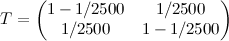 ;
;- E = (N (0.1), N (0.1.21)).
Let us find the most plausible states for each moment of time using the Viterbi algorithm for the given model parameters.
The solution of the problem is reduced to specifying the model and running the Viterbi algorithm.
Using the model of hidden Markov chains and a sample of values of the observed characteristics, we find the sequence of states that best describes the sample in a given model. The concept can best be interpreted differently, but the well-established solution is the Viterbi algorithm, which finds such a sequence
, what .Search task
is solved using dynamic programming, for this we consider the function:Where
- the highest probability of being able to s at the moment of time t. Recursively, this function can be defined as follows:Simultaneously with the calculation
for each moment of time we remember the most probable state from which we came, that is, at which the maximum was reached. Wherein and that means you can recover , walking on them in reverse order. You may notice that - the value of the desired probability. Required sequence found. An interesting feature of the algorithm is that the estimated function of the observed characteristics is included in in the form of a factor. If we assume that , then in the case of omissions in observations, it is still possible to estimate the most probable hidden states at these moments.The “Pseudocode” for the Viterbi algorithm is sketched below. It should be noted that all operations with vectors and matrices are element-wise .
Tm<-10000 # Max time M<-2 # Number of states S<-seq(from=1, to=M) # States [1,2] I<-rep(1./M, each=M) # Initial distribution [0.5, 0.5] T<-matrix(c(1-4./Tm, 4./Tm, 4./Tm,1-4./Tm),2) #[0.9995 0.0005; 0.0005 0.9995] P<-c(function(o){dnorm(o)}, function(o){dnorm(o,sd=1.1)}) # Vector of density functions for each state (N(0,1), N(0,1.21)) E<-function(P,s,o){P[[s]](o)} # Calculate probability of observed value o for state s. Es<-function(E,P,o) { # Same for all states probs<-c() for(s in S) { probs<-append(probs, E(P,s,o)) } return(probs) } viterbi<-function(S,I,T,P,E,O,tm) { delta<-I*Es(E,P,O[1]) # initialization for t=1 prev_states<-cbind(rep(0,length(S))) # zeros for(t in 2:Tm) { m<-matrix(rep(delta,length(S)),length(S))*T # delta(s')*T[ss'] forall s,s' md<-apply(m,2,max) # search for max delta(s) by s' for all s max_delta<-apply(m,2,which.max) prev_states<-cbind(prev_states,max_delta) delta<-md*Es(E,P,O[t]) # prepare next step delta(s) } return(list(delta=delta,ps=prev_states)) # return delta_Tm(s) and paths } restoreStates<-function(d,prev_states) { idx<-which.max(d) s<-c(idx) sz<-length(prev_states[1,]) for(i in sz:2) { idx<-prev_states[idx,i] s<-append(s,idx,after=0) } return (as.vector(s)) } Someone could recognize the code in R in this “pseudocode”, but this is far from the best implementation.
Let us compare the periods of constancy of the states that were specified in the simulation (the upper part of the graph) and those that were found using the Viterbi algorithm (the lower part of the graph):
It is quite worthy in my opinion, but every time you should not hope for that.
The previously described Viterbi algorithm requires the definition of a hidden Markov chain model (Arguments of the viterbi function). To set them, a simple initialization is used, which implies that in addition to a sample of observable quantities O, a corresponding selection of hidden states Q, which we know from somewhere, is also given. In this case, the formulas for estimating the parameters will be as follows:
where Id (x) is an indicator function,
For the considered lie detector example, the algorithm incorrectly classified 413 out of 10,000 states (~ 4%), which is not bad at all. The Viterbi algorithm is able to accurately detect the moments of change of hidden states, but only if the distributions of the observed characteristics are accurately known. If only a parametric class of such distributions is known, then there is a way to select the most appropriate parameters, called the Baum-Welch algorithm.
If interested, ask to continue ...
Source: https://habr.com/ru/post/180109/
All Articles