Creating a single routing offline and online products 2GIS
If someone else does not know, then 2GIS is a free directory of organizations with a city map. And if a lot has already been written about the directory , then there is less information about the map and its capabilities. And there is something to tell. For example, about routing - why we did not take existing solutions, but wrote our own or why we need a single algorithm for building in different products.
In early 2012, we first encountered a problem - the engine that was previously used in the desktop version turned out to be too demanding of resources and cannot be used on mobile devices . It was necessary to do something.
')
Why not take ready-made solutions?
It is believed that the routing engine is a very difficult task with a lot of subtleties of implementation. It’s as if you don’t go into boost :: graph and you don’t need to take it (it’s not supposed to know about the movie, yes) and it’s easier to find a ready-made solution. Perhaps, but not in our case.
I hope that it will become clear from the article - common sense, a bit of adventurism and a guide that is ready for the whole allow to solve any problem.
In fairness, it should be noted that I already had experience with search in graphs (~ 50 million vertices), so some ideas about how to solve such problems already existed.
So, introductory:
Let's designate the main (and, banal, in general) principles :
Main ideas
Initial data
Pretreatment
Disk storage
The actual data is stored in B-trees, more precisely in one of their varieties.
From the data warehouse, we need the ability to store a sorted N-ok array and quickly read their intervals.
By and large, the choice of storage is not critical, we chose B-trees, because they:
So, there are several trees:
1. Tree tops. N-ka of this tree consists of 4 elements:
2. Edge tree , His key consists of 7 elements:
3. Tree of identifiers. Used to communicate with the outside world. The key contains 5 items:
4. Tree of restrictions with a key of length 4:
Thoughtful reader will say: “Bah! To read all the information about a single tile, you need to make 3 lines of trees. Isn't it better to pack everything into a BLOB and pick it up in one fell swoop? ”For read-only data, it’s better, of course, in terms of speed and compression quality. But this is additional work, additional testing. In addition, profiling showed that, in fact, the reading of data is not a bottleneck when searching for directions.
If we are talking about data that can dynamically change, here B-trees are out of competition. It is not even necessary to have your own implementation of trees, you can use SQL storage, and set the above-described entities as tables consisting of only primary key. So, one of the predecessors of the described engine was built on the basis of OpenLink Virtuoso DBMS, where the tables themselves are arranged like trees and, in our case, there is no duplication of data as such (meaning duplication of data from the table in the index).
Graph representation in memory
In this section we describe how the unpacked graph looks in memory.
1. The entire graph in memory may not exist. As already mentioned, it is loaded slowly as someone needs parts of this graph.
2. Therefore, there is a cache of tiles and a holder of this cache. Caching strategy can be any. We have this LRU (Least Recently Used).
3. Tile loaded into memory - contains all the information about the data trapped in its area of space. As already mentioned, all the memory for this is allocated from the tile-owned allocator and is released upon its death. Namely:
4. Thus, a tile in memory is a ready-to-use piece of the graph that can:
Actually search
1. Before starting the search, you need to bind to the graph. Those. on the outside we get two sets of points - the source and the end. The description of each point consists of its external identifier of the graph edge and cost. The cost of reaching the beginning of this edge for the starting point and the cost of the path from the end of the edge to the final for the ending point. So:
2. Using the tree of identifiers, we turn edge identifiers into entry points to the graph (const vertex_t *). To do this, you will need to contact the tile cache holder and load the necessary ones.
We need an object - the holder of information about the final, including tile identifiers and vertex numbers. Another useful information that this object possesses is the geometrical position of the finish. It can be given explicitly, but it can be calculated, for example, as the centroid of the final points. We will need this point to calculate the estimated part of the cost of the reached vertex for the algorithm A *
3. Now we need a “wave” holder. It consists of:
a. Allokator, well, where can I go without it.
b. A set of loaded tiles. For graphs of reasonable size, a bit mask is sufficient. That is, when we hit a tile for the first time, mark the corresponding bit in this mask and increment the counter of its links. After completing the search, focusing on this mask, we will roll back the reference counters. At the same time, those tiles whose counters have been reset will receive a chance to fly out of the cache in the future.
c. Priority queue. We use a binary sorting heap. Candidates for viewing are in the queue. For example, starting points go straight here. The key here is the distance traveled or the time spent. And the value is a pointer to the handle of the passed point.
d. Set of points passed. Each such point is described by a structure:
Of course, these structures are allocated with an allocator.
4. So, for each starting point, we create its descriptor and put it in a heap. So we are ready to start the search.
5. While there is something in the heap (and so far it is something potentially better than the already found candidates), choose the cheapest element from it and:
a. we run according to the list of its outgoing edges and for each of them:
I. check the possibility of transition to this edge from the previous one.
Ii. find the vertex of the graph pointed to by this edge. It is possible that a new tile will be loaded, and this point will be in it.
III.Calculate the cost of achieving this new point. For this:
Iv. create and fill the handle of the traversed vertex
V. check whether this is final
Vi. if it is a finish, then we unwind the list of previous ones
(vertex_ptr_t :: prev_) , starting from this point, while on the rest in 0,
those. at the start Here is a ready candidate for extradition.
VII. we put the created descriptor in a heap
results
Let's try to evaluate the results of the deed on the example of the road graph of the capital of our vast Motherland.
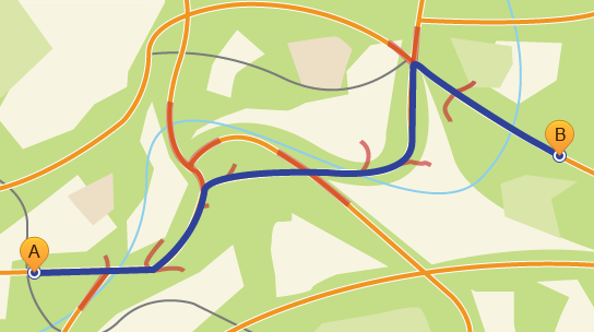
Blue indicates the optimal route, red - “wave”.
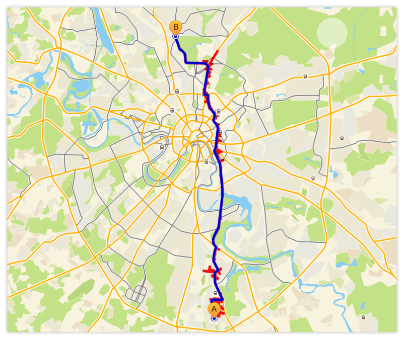
As before, blue is the optimal route, red is the “wave”.
It's funny to see how the search revealed (actual, implicit) hierarchical structure of the graph and began to use it.

Total
As we can see, such a simple data structure and the described algorithm allow you to work with a single-level graph of a big city on an ordinary smartphone. And if RAM allows us, for example, in the server case, increasing the size of the tile cache, we simply drive the entire graph into memory and work with its ready representation. That has a beneficial effect on performance.
We intentionally did not touch on certain points, for example, taking into account the traffic situation, prediction of this, hierarchical graphs, because this is a completely different story.
That's All Folks!
In early 2012, we first encountered a problem - the engine that was previously used in the desktop version turned out to be too demanding of resources and cannot be used on mobile devices . It was necessary to do something.
')
Why not take ready-made solutions?
It is believed that the routing engine is a very difficult task with a lot of subtleties of implementation. It’s as if you don’t go into boost :: graph and you don’t need to take it (it’s not supposed to know about the movie, yes) and it’s easier to find a ready-made solution. Perhaps, but not in our case.
I hope that it will become clear from the article - common sense, a bit of adventurism and a guide that is ready for the whole allow to solve any problem.
In fairness, it should be noted that I already had experience with search in graphs (~ 50 million vertices), so some ideas about how to solve such problems already existed.
So, introductory:
- In the server version, the same code should work, but with different settings;
- Building a path should work on mobile phones for a reasonable time;
- In the asset ready (and verified) road graph; It turned out to be much easier / more convenient / cheaper than searching and sharpening ready-made solutions.
Let's designate the main (and, banal, in general) principles :
- Storage structures should be simple.
- It is useful to stimulate the locality of links, i.e. if the data is related to physically close (for example) vertices of the graph, then they should be located nearby on the disk if possible.
- In no case should the elements of the graph on the disk be addressed one at a time, reading is carried out only in batches.
- Low-level caching is of little use, you should only care about “expensive” objects. For example, instead of directly caching disk accesses, it is better to take care to minimize their number in an algorithmic way.
- The search logic in the graph should be simplified, where it is possible, because “if breaks the conveyor” (C)
- Compress the data on the disk - good.
- It is not reprehensible to disregard precision in favor of performance.
Main ideas
- Put the coordinates of the vertices on the lattice. Those. translate floating point coordinates into integers. The grid can be made rather coarse, increasing its pitch until the vertices begin to stick together or, worse, to form edges of zero length. When searching, we will need the coordinates to estimate the remaining distance to the final (and for debugging) and with the lattice with a large step, not far from the finish, the algorithm will start to behave strangely.
Note that the rougher the grating, the smaller the amount of data on the disk, so if you really want it, you can choose it iteratively. We have a lattice step - meter.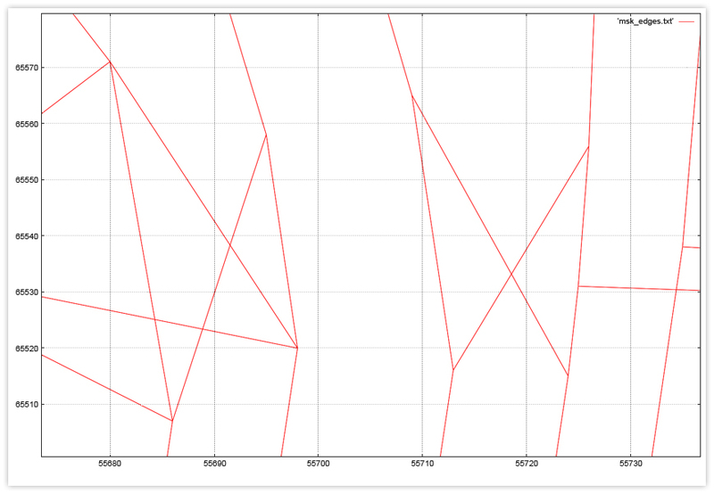
Here is a fragment of a graph planted on a grid. - Mentally divide the extent of our graph into a number of rectangular tiles that form a grid. This lattice does not have to be a sublattice thereof at the vertices.
- A tile is a logical unit to be simultaneously loaded from disk and cached. It contains all vertices and outgoing arcs (i.e. arcs whose initial vertices lie in this tile). Plus related information, if any.

An example of edges that fell into one tile using the example of a fragment of a Moscow road graph. - The size of the tile should be selected based on the size of the graph. Once we load something from the disk, it will be reasonable that the total amount of information read is comparable with the size of the disk buffer. It would be strange to use heavy artillery in the form of disk hits to access several peaks that fit in a hundred bytes. Of course, the graph is unevenly arranged, but you can appeal to average values, for example, the graph occupies 20mb on the disk, i.e. 2500 8K pages, hence sawing the extent of the graph into 50 × 50 parts (sqrt (2500)). Here it is implicitly assumed that all information about the tile lies in one place. If this is not the case, an appropriate amendment must be made.
- It makes sense to cache it tiles.
- A graph loaded into memory (or its part) is a large number of small objects. It is impossible with impunity to allocate and release large quantities of small objects. Therefore, we will use session page allocators, where possible. In addition to speed and much less fragmentation of memory, this will also provide savings on the prologue and epilogue of the data block (meaning an algorithm with double tags).
A page allocator distributes memory from its fixed-size pages (if possible), which it solicits from the system as needed. Memory is released only all at once in its destructor. - A tile will necessarily have such an allocator, everything that will be allocated when it is loaded will be taken from it and will die with its tile when it is pushed out of the cache.
- Another candidate for the use of the page allocator is the search itself, it is convenient to store information about the passed part of the graph in this way.
- Actually search algorithm. We will use an ordinary A *, one “wave”, with an estimate of the value of the vertex as the sum of the distance traveled (or time) and the estimate of the remaining one.
- A * - because It allows you to reduce the number of traversed vertices compared to the original Dijkstra algorithm.
- One wave - for two reasons. First, the launch of two waves towards meet, although it reduces the portion of the graph, but it will complicate the stopping criterion because we must constantly check whether two waves are encountered. And this entails either the content of each wave of a dynamic set of traversed vertices, or a modification of directly loaded tiles.
- The second reason is that the presence of an oncoming wave will not allow dynamically influencing the cost of the ribs, for example, due to a change in the traffic situation by the time we mentally get to this edge.
- The estimate of the cost of the remaining path can be any, provided that the triangle inequality is not violated. For example, you can use a fair Euclidean distance or Chebyshev distance.
Initial data
- Graph vertices - structures having coordinates and identifier
- Edges contain the identifier, length, type and identifiers of the initial and final vertices. All edges are unidirectional.
- Restrictions - a pair of edges, the transition between which is impossible. The constraint is tied to a specific vertex common to both edges. We describe such a rather truncated version of the restrictions; if necessary, the reader will easily come up with a generalization.
Pretreatment
- Find the inclusive extent of the graph.
- We determine the lattice coordinates.
- We are determined with a grid of tiles. Each tile is assigned its ID. The identifier is the number that grows as a result of the work of some sweeping curve. Such a curve can be a line scan (igloo), a Hilbert curve, or a bit interleaving curve (zorder). By and large, it is only important to be able to determine, by the coordinates of a point, which tile it falls into. And the choice of a sweeping curve only affects the ability of the data to be compressed.
- We assign each vertex to a specific tile. In this case, we assign each vertex its ordinal number in its tile, this is also useful for compression.
- For each edge, we determine which tile it goes from and into which tile, as well as the internal numbers of the outgoing and incoming points.
Disk storage
The actual data is stored in B-trees, more precisely in one of their varieties.
From the data warehouse, we need the ability to store a sorted N-ok array and quickly read their intervals.
By and large, the choice of storage is not critical, we chose B-trees, because they:
- Easy to understand and debug
- Allow to compress data without being tied to specific
- Most importantly, their implementation was tested at hand.
So, there are several trees:
1. Tree tops. N-ka of this tree consists of 4 elements:
- Vertex Tile ID
- The ordinal number of the vertex in this tile
- X - point coordinate
- Y is the coordinate of the point.
2. Edge tree , His key consists of 7 elements:
- Outgoing vertex tile identifier
- Number of outgoing vertex in its tile
- Incoming vertex tile identifier
- The number of the incoming vertex in its tile
- Edge cost, for example, length
- Edge type, for example, road class
- External identifier of the edge.
3. Tree of identifiers. Used to communicate with the outside world. The key contains 5 items:
- External edge ID
- Outgoing vertex tile number
- Number of outgoing vertex in its tile
- Tile number of the incoming vertex
- The number of the incoming vertex in its tile.
4. Tree of restrictions with a key of length 4:
- The tile number of the vertex of the constraint.
- The number of this vertex in the tile
- External identifier of the edge from which movement is prohibited
- External identifier of the edge where movement is prohibited.
Thoughtful reader will say: “Bah! To read all the information about a single tile, you need to make 3 lines of trees. Isn't it better to pack everything into a BLOB and pick it up in one fell swoop? ”For read-only data, it’s better, of course, in terms of speed and compression quality. But this is additional work, additional testing. In addition, profiling showed that, in fact, the reading of data is not a bottleneck when searching for directions.
If we are talking about data that can dynamically change, here B-trees are out of competition. It is not even necessary to have your own implementation of trees, you can use SQL storage, and set the above-described entities as tables consisting of only primary key. So, one of the predecessors of the described engine was built on the basis of OpenLink Virtuoso DBMS, where the tables themselves are arranged like trees and, in our case, there is no duplication of data as such (meaning duplication of data from the table in the index).
Graph representation in memory
In this section we describe how the unpacked graph looks in memory.
1. The entire graph in memory may not exist. As already mentioned, it is loaded slowly as someone needs parts of this graph.
2. Therefore, there is a cache of tiles and a holder of this cache. Caching strategy can be any. We have this LRU (Least Recently Used).
3. Tile loaded into memory - contains all the information about the data trapped in its area of space. As already mentioned, all the memory for this is allocated from the tile-owned allocator and is released upon its death. Namely:
struct vertex_t {int x_; int y_; const link_t*links_; }; , .. . links_ , . struct link_t { int64_tfid_; // int len_; // int class_; // int vert_id_; // , >0, union { const vertex_t *vertex_; // int tile_id_; // }; const link_t *next_; // }; struct restriction_t {uint64_t from_; uint64_t to_;}; . , ( ) . , . 4. Thus, a tile in memory is a ready-to-use piece of the graph that can:
- Give vertex by number
- Verify outgoing edges by vertex
- Test a couple of edges for restrictions on it.
- Edges are either pointers when moving inside a tile, or a pair of tile number / vertex number otherwise. For this pair, when moving along the graph, you can transparently ask the required cache holder for the cache holder, load it if necessary, and switch to it.
Actually search
1. Before starting the search, you need to bind to the graph. Those. on the outside we get two sets of points - the source and the end. The description of each point consists of its external identifier of the graph edge and cost. The cost of reaching the beginning of this edge for the starting point and the cost of the path from the end of the edge to the final for the ending point. So:
2. Using the tree of identifiers, we turn edge identifiers into entry points to the graph (const vertex_t *). To do this, you will need to contact the tile cache holder and load the necessary ones.
We need an object - the holder of information about the final, including tile identifiers and vertex numbers. Another useful information that this object possesses is the geometrical position of the finish. It can be given explicitly, but it can be calculated, for example, as the centroid of the final points. We will need this point to calculate the estimated part of the cost of the reached vertex for the algorithm A *
3. Now we need a “wave” holder. It consists of:
a. Allokator, well, where can I go without it.
b. A set of loaded tiles. For graphs of reasonable size, a bit mask is sufficient. That is, when we hit a tile for the first time, mark the corresponding bit in this mask and increment the counter of its links. After completing the search, focusing on this mask, we will roll back the reference counters. At the same time, those tiles whose counters have been reset will receive a chance to fly out of the cache in the future.
c. Priority queue. We use a binary sorting heap. Candidates for viewing are in the queue. For example, starting points go straight here. The key here is the distance traveled or the time spent. And the value is a pointer to the handle of the passed point.
d. Set of points passed. Each such point is described by a structure:
struct vertex_ptr_t { int64_t fid_; // , // 0 const vertex_t *ptr_; // const vertex_ptr_t *prev_; // size_t cost_len_; // size_t cost_time_; // }; Of course, these structures are allocated with an allocator.
4. So, for each starting point, we create its descriptor and put it in a heap. So we are ready to start the search.
5. While there is something in the heap (and so far it is something potentially better than the already found candidates), choose the cheapest element from it and:
a. we run according to the list of its outgoing edges and for each of them:
I. check the possibility of transition to this edge from the previous one.
Ii. find the vertex of the graph pointed to by this edge. It is possible that a new tile will be loaded, and this point will be in it.
III.Calculate the cost of achieving this new point. For this:
- take the accumulated path and time
- sum up the path with the length of the current edge
- we increase the time by the amount needed to overcome the current in accordance with its length, type and anything else
- we calculate and add the estimate of the remaining path - abs (dx) + abs (dy), where dx and dy - the difference in longitude and latitude, respectively
- we calculate and add an estimate of the time remaining to the finish based on the estimate of the remaining path, time of day, average speed on
- passed stage and anything else
Iv. create and fill the handle of the traversed vertex
V. check whether this is final
Vi. if it is a finish, then we unwind the list of previous ones
(vertex_ptr_t :: prev_) , starting from this point, while on the rest in 0,
those. at the start Here is a ready candidate for extradition.
VII. we put the created descriptor in a heap
results
Let's try to evaluate the results of the deed on the example of the road graph of the capital of our vast Motherland.
- The graph contains 307338 vertices
- And 806220 ribs.
- The size of the extent - 92 x 112 km
- Number of tiles - 46 x 56 = 2576 pieces
- The total amount of data on the disk occupied by the road graph is 13 980 kb
- The average length of the calculated path is 32.8 km
- For example,
Blue indicates the optimal route, red - “wave”.
- In this case, on average, 1644 vertices and 2406 edges are covered, which lie on 22 tiles.
- This requires 2096 kb for tiles and 116 kb for wave
- time spent on Sony Xperia S 400 + 500 (on index initialization) ms (IPhone 4 800 + 1000 (...) ms)
- Example, the path through the entire graph
As before, blue is the optimal route, red is the “wave”.
It's funny to see how the search revealed (actual, implicit) hierarchical structure of the graph and began to use it.
- Its calculated length is 135.3 km.
- This affects 2251 vertices and 3044 edges, lying on 120 tiles.
- This requires 3,946 kb for tiles and 133 kb for wave
- time spent 400 ms Sony Xperia S (500 IPhone 4) plus the same one-time index load, of course
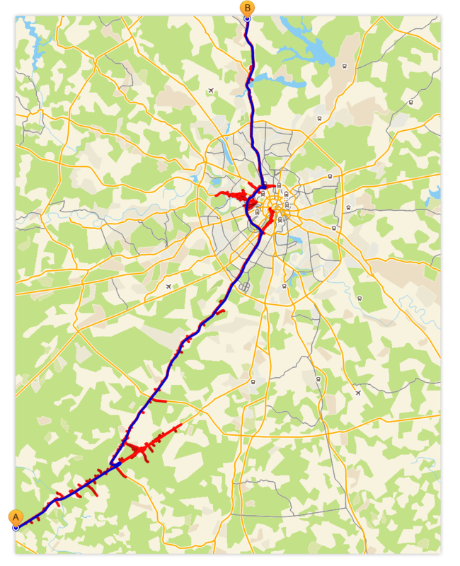
- And here is a demonstration of how important the heuristics used are - three pictures of a passage in Novosibirsk with different settings:
Total
As we can see, such a simple data structure and the described algorithm allow you to work with a single-level graph of a big city on an ordinary smartphone. And if RAM allows us, for example, in the server case, increasing the size of the tile cache, we simply drive the entire graph into memory and work with its ready representation. That has a beneficial effect on performance.
We intentionally did not touch on certain points, for example, taking into account the traffic situation, prediction of this, hierarchical graphs, because this is a completely different story.
That's All Folks!
Source: https://habr.com/ru/post/179749/
All Articles